rtestim Package Vignette • rtestim

library(rtestim)
library(ggplot2)
theme_set(theme_bw())

Overview

This package uses Poisson likelihood with trend filtering penalty (a type of regularized nonparametric regression) to estimate the effective reproductive number, $R_t$ . This value roughly says “how many new infections will result from each new infection today”. Values larger than 1 indicate that an epidemic is growing while those less than 1 indicate decline.

This vignette provides a few examples to demonstrate the usage of rtestim to estimate the effective reproduction number, $R_t$ . rtestim finds a sequence of $R_t$ , $\{R_t\}_{t=1}^n$ of an infectious disease by solving the following penalized Poisson regression $\begin{equation} \label{eq:objective_fn} \hat{\theta} = \mathop{\mathrm{argmin}}_{\theta} \frac{1}{n} \sum_{t=1}^n \left(e^{\theta_{t}}x_t - y_t\theta_{t}\right) + \lambda \Vert D^{(k+1)} \theta \Vert_1 \end{equation}$ where $y_t$ is the an epidemic signal, ideally, incident infections, but most frequently, incident cases, on day $t$ , $\theta_{t} = \log(R_t)$ is the natural logarithm of $R_t$ at time $t$ , $D^{(k)}$ is the $k$ -th order divided difference operator ( $k \geq 0$ ). The penalty $\Vert D^{(k+1)} \theta \Vert_1$ imposes smoothness on the solution and $\lambda$ controls the level of this smoothness, with larger $\lambda$ resulting in smoother estimates.

In particular $\begin{equation} x_t = \sum_{a = 1}^m y_{t-a} w_a \end{equation}$ is the weighted sum of previous incidence at $t$ , calculated by convolving the preceding $m$ days of new infections with the discretized serial interval distribution $w$ of length $m$ . This delay distribution encapsulates the duration of time that a previous infection is likely to lead to future infection.

To compute $\{R_t\}_{t=1}^n$ with rtestim, the minimal information needed is the new case counts at days up until $t$ and a parametric form for the serial interval distribution (a Gamma density). By default, $2.5$ is used for both the scale and shape parameters, based on the literature on contract tracing, representing the typical delay between case onsets. This is discretized to be supported on the integers. The order of the difference operator, the degree of smoothness, defaults to $3$ . The sequence of smoothness penalty $\lambda$ , if no $\lambda$ is provided, is calculated internally by the algorithm.

Example - synthetic dataset

Quick start

We first demonstrate the usage of the package on synthetic data, where the new daily case counts are generated from a Poisson distribution with mean parameter that roughly follows a wave. Note that the first observation must be strictly larger than 0.

set.seed(12345)
case_counts <- c(1, rpois(100, dnorm(1:100, 50, 15) * 500 + 1))
ggplot(data.frame(x = 1:101, case_counts), aes(x, case_counts)) +
  geom_point(colour = "cornflowerblue") +
  labs(x = "Time", y = "Case Counts")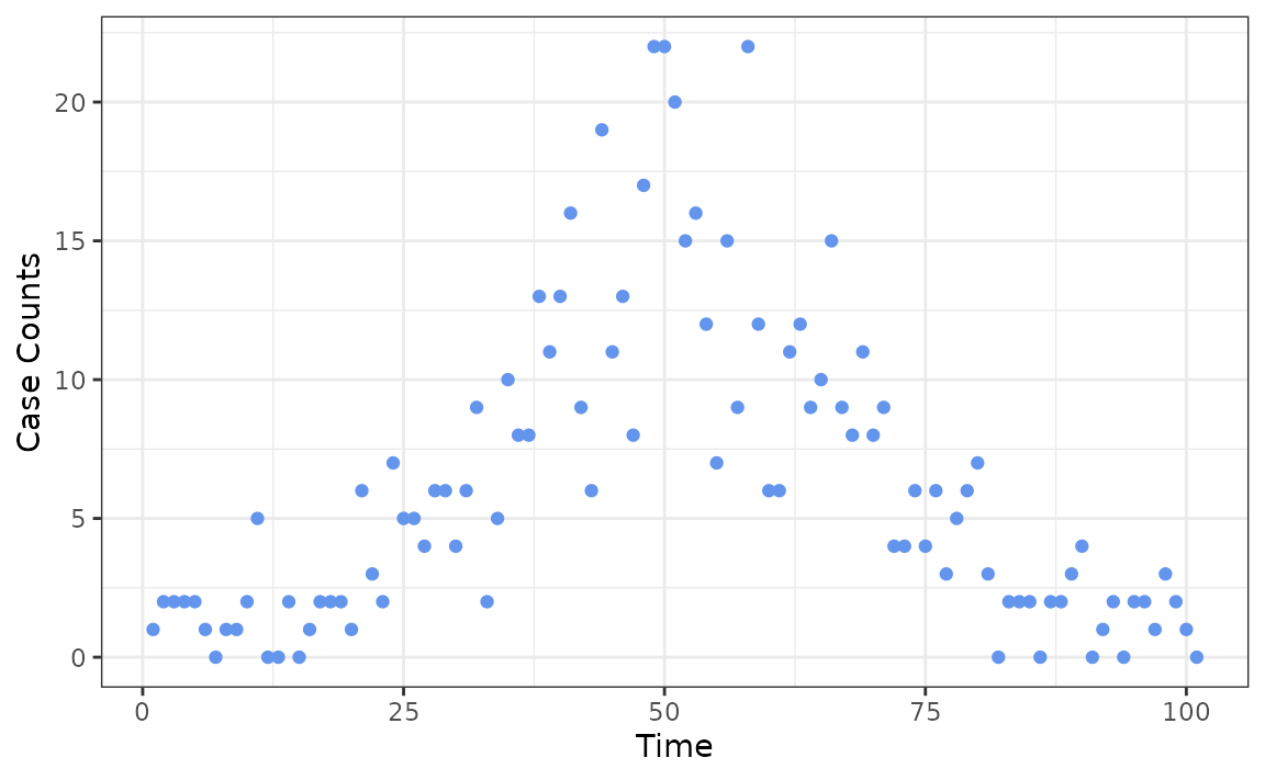

Next, we fit the model and visualize the resulting $\{R_t\}_{t=1}^n$ :

mod <- estimate_rt(observed_counts = case_counts, nsol = 20)
plot(mod)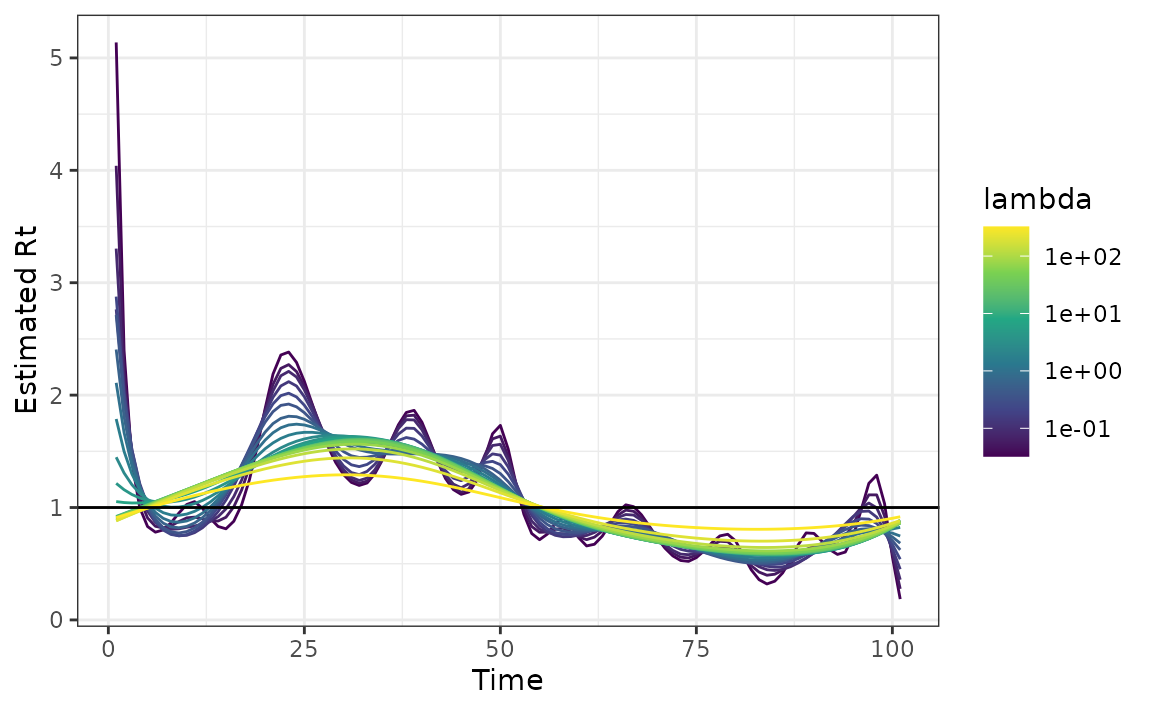

rtestim estimates a spectrum of $\{R_t\}_{t=1}^n$ s for a range of $\lambda$ values, where each $\{R_t\}_{t=1}^n$ corresponds to a specific $\lambda$ value. If no $\lambda$ value is supplied by the user, rtestim will automatically calculate a sequence of $\lambda$ values. The additional parameter nsol = 20 specifies the number of $\lambda$ s for which the $\{R_t\}_{t=1}^n$ is calculated

Cross Validation

rtestim also provides a cross validation procedure for selecting the amount of smoothness to be used in the final estimate (leave-every-k-th-out cross validation). Minimizing this metric, in principle, balances prediction error and smoothness (lambda.min) though if smoother estimates are desired, one can instead use lambda.1se, the largest value of $\lambda$ within one standard error of the minimum.

mod_cv <- cv_estimate_rt(observed_counts = case_counts)

The following command plots the cross validation errors for each $\lambda$ in ascending order.

plot(mod_cv)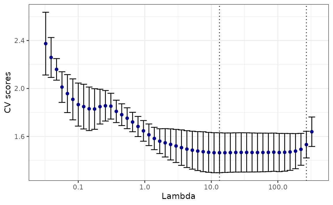

The plot above displays vertical lines that correspond to the cross-validation scores for specific values of $\lambda$ . The blue point at the center of each line represents the mean score for that value of $\lambda$ across all cross-validation folds. The top and bottom caps of each line indicate one cross-validation standard error above and below the mean score for the given value of $\lambda$ across all cross-validation folds. Two special values of $\lambda$ ’s are highlighted with dashed lines. The one on the left represents the $\lambda$ that gives minimum mean cross-validated error, called lambda.min, and the one on the right gives the most regularized model such that the cross-validated error is within one standard error of the minimum, called lambda.1se.

Users may wish to visualize the particular $\{R_t\}_{t=1}^n$ which minimizes the cross-validation error while prioritizing smoothness.

plot(mod_cv, which_lambda = "lambda.1se")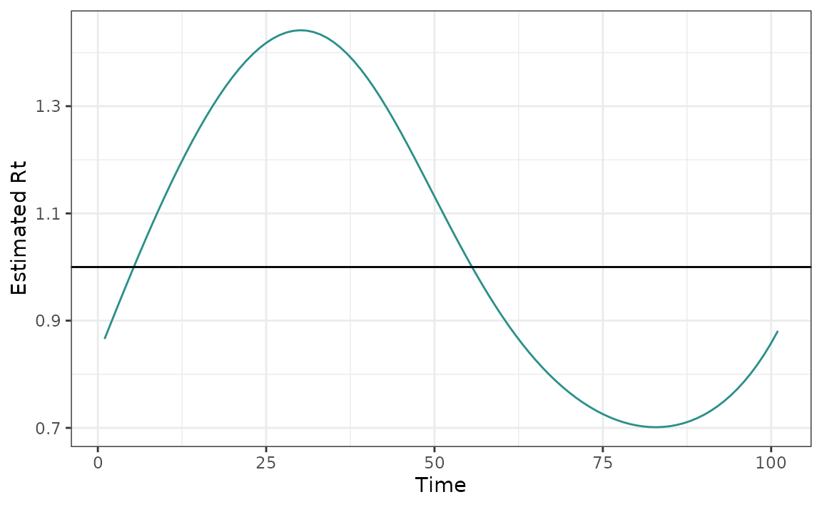

Uneven Reporting Frequency

Ideally, case counts are observed at regular intervals, such as daily or weekly, but this is not always the case. rtestim also accommodates scenarios in which cases are reported with uneven intervals. To demonstrate this, we generate a sequence of integers representing the days at which we observe the case counts.

observation_incr <- rpois(101, lambda = 2)
observation_incr[observation_incr == 0] <- 1
observation_time <- cumsum(observation_incr)

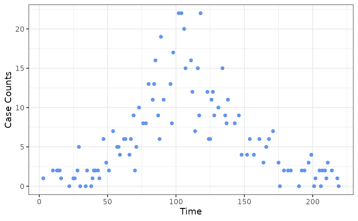
We can then fit the model by passing the observation time point as x.

mod <- estimate_rt(observed_counts = case_counts, x = observation_time)
plot(mod)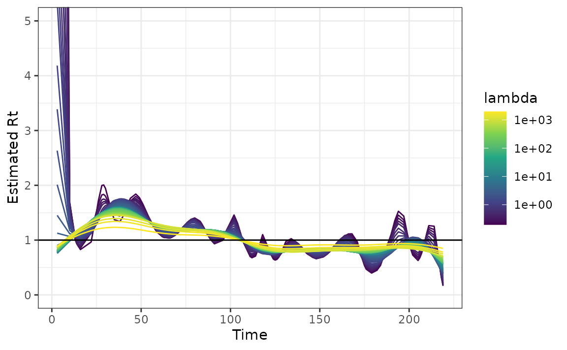 + coord_cartesian(ylim = c(0, 5))

Changing degree of difference operator

The degree of the estimated penalized Poisson regression function $k$ defaults to 3 for the algorithm, which corresponds to a piece-wise cubic estimate $\{R_t\}_{t=1}^n$ . To estimate $\{R_t\}_{t=1}^n$ with piece-wise constant curves for example, use the command

mod <- estimate_rt(observed_counts = case_counts, korder = 0, nsol = 20)
plot(mod)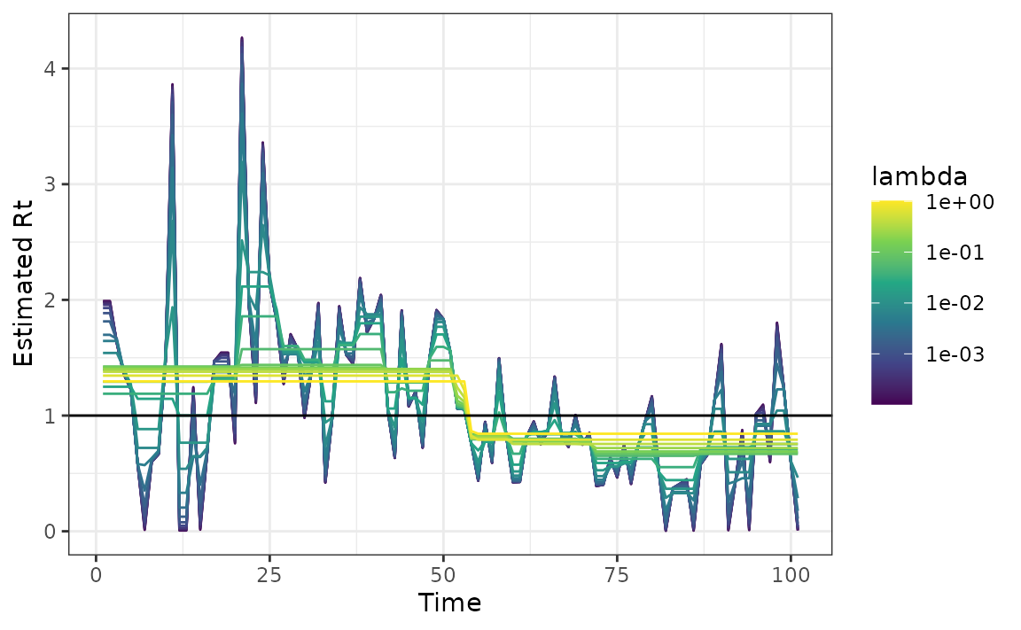

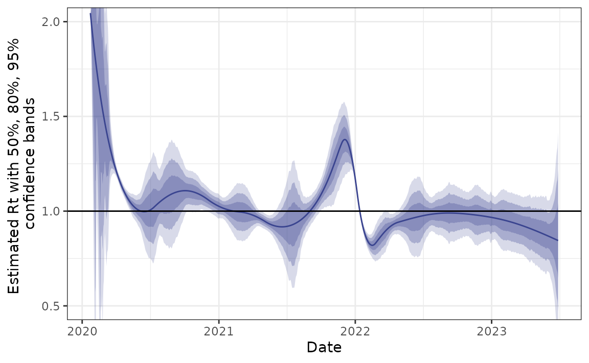
Example - Canadian Covid-19 cases

Finally, we use a long history of real case counts in Canada. The data is available from opencovid.ca and the version downloaded on 4 July 2023 is included in the package. We use this data to estimate $R_t$ .

can <- estimate_rt(
  observed_counts = cancovid$incident_cases,
  x = cancovid$date,
  korder = 2,
  nsol = 20,
  maxiter = 1e5
)

plot(can) + coord_cartesian(ylim = c(0.5, 2))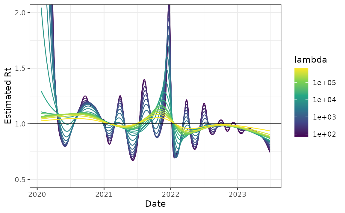

Approximate confidence bands

We also provide functionality for computing approximate confidence bands for Rt based on normal approximations and the delta method. These are intended to be fast and to provide some idea of uncertainty, but they likely don’t have guaranteed coverage.

can_cb <- confband(can, lambda = can$lambda[10], level = c(.5, .8, .95))
can_cb

#> An `rt_confidence_band` object.
#> 
#> * type = Rt 
#> * lambda = 8976.305 
#> * degrees of freedom = 12 
#> 
#> # A tibble: 1,253 × 7
#>      fit  `2.5%` `10.0%` `25.0%` `75.0%` `90.0%` `97.5%`
#>    <dbl>   <dbl>   <dbl>   <dbl>   <dbl>   <dbl>   <dbl>
#>  1  2.05 NaN      NaN     NaN     NaN     NaN     NaN   
#>  2  2.03   1.95     1.97    2.00    2.05    2.08    2.10
#>  3  2.01   1.85     1.91    1.95    2.06    2.11    2.16
#>  4  1.99   1.74     1.83    1.90    2.07    2.15    2.23
#>  5  1.97   1.60     1.73    1.84    2.09    2.21    2.33
#>  6  1.95   1.44     1.62    1.77    2.12    2.28    2.45
#>  7  1.93   1.27     1.50    1.70    2.16    2.36    2.59
#>  8  1.91   1.09     1.38    1.63    2.19    2.45    2.73
#>  9  1.89   0.918    1.26    1.56    2.23    2.53    2.87
#> 10  1.88   0.756    1.14    1.49    2.26    2.61    3.00
#> # ℹ 1,243 more rows

plot(can_cb) + coord_cartesian(ylim = c(0.5, 2))