Estimate Rt using smoothness-penalized Poisson likelihood

The Effective Reproduction Number $R_t$ of an infectious disease can be estimated by solving the smoothness penalized Poisson regression (trend filtering) of the form:

$$\hat{\theta} = \arg\min_{\theta} \frac{1}{n} \sum_{i=1}^n (w_i e^{\theta_i} - y_i\theta_i) + \lambda\Vert D^{(k+1)}\theta\Vert_1, $$

where $R_t = e^{\theta}$, $y_i$ is the observed case count at day $i$, $w_i$ is the weighted past counts at day $i$, $\lambda$ is the smoothness penalty, and $D^{(k+1)}$ is the $(k+1)$-th order difference matrix.

Usage

estimate_rt(
  observed_counts,
  korder = 3L,
  dist_gamma = c(2.5, 2.5),
  x = 1:n,
  lambda = NULL,
  nsol = 50L,
  delay_distn = NULL,
  delay_distn_periodicity = NULL,
  lambdamin = NULL,
  lambdamax = NULL,
  lambda_min_ratio = 1e-04,
  maxiter = 1e+05,
  init = configure_rt_admm()
)

Arguments

observed_counts: vector of the observed daily infection counts
korder: Integer. Degree of the piecewise polynomial curve to be estimated. For example, korder = 0 corresponds to a piecewise constant curve.
dist_gamma: Vector of length 2. These are the shape and scale for the assumed serial interval distribution. Roughly, this distribution describes the probability of an infectious individual infecting someone else after some period of time after having become infectious. As in most literature, we assume that this interval follows a gamma distribution with some shape and scale.
x: a vector of positions at which the counts have been observed. In an ideal case, we would observe data at regular intervals (e.g. daily or weekly) but this may not always be the case. May be numeric or Date.
lambda: Vector. A user supplied sequence of tuning parameters which determines the balance between data fidelity and smoothness of the estimated Rt; larger lambda results in a smoother estimate. The default, NULL results in an automatic computation based on nlambda, the largest value of lambda that would result in a maximally smooth estimate, and lambda_min_ratio. Supplying a value of lambda overrides this behaviour. It is likely better to supply a decreasing sequence of lambda values than a single (small) value. If supplied, the user-defined lambda sequence is automatically sorted in decreasing order.
nsol: Integer. The number of tuning parameters lambda at which to compute Rt.
delay_distn: in the case of a non-gamma delay distribution, a vector or matrix (or Matrix::Matrix()) of delay probabilities may be passed here. For a vector, these will be coerced to sum to 1, and padded with 0 in the right tail if necessary. If a time-varying delay matrix, it must be lower-triangular. Each row will be silently coerced to sum to 1. See also vignette("delay-distributions").
delay_distn_periodicity: Controls the relationship between the spacing of the computed delay distribution and the spacing of x. In the default case, x would be regular on the sequence 1:length(observed_cases), and this would be 1. But if x is a Date object or spaced irregularly, the relationship becomes more complicated. For example, weekly data when x is a date in the form YYYY-MM-DD requires specifying delay_distn_periodicity = "1 week". Or if observed_cases were reported on Monday, Wednesday, and Friday, then delay_distn_periodicity = "1 day" would be most appropriate.
lambdamin: Optional value for the smallest lambda to use. This should be greater than zero.
lambdamax: Optional value for the largest lambda to use.
lambda_min_ratio: If neither lambda nor lambdamin is specified, the program will generate a lambdamin by lambdamax * lambda_min_ratio. A multiplicative factor for the minimal lambda in the lambda sequence, where lambdamin = lambda_min_ratio * lambdamax. A very small value will lead to the solution Rt = log(observed_counts). This argument has no effect if there is a user-defined lambda sequence.
maxiter: Integer. Maximum number of iterations for the estimation algorithm.
init: a list of internal configuration parameters of class rt_admm_configuration.

Value

An object with S3 class poisson_rt. Among the list components:

observed_counts the observed daily infection counts.
x a vector of positions at which the counts have been observed.
weighted_past_counts the weighted sum of past infection counts.
Rt the estimated effective reproduction rate. This is a matrix with each column corresponding to one value of lambda.
lambda the values of lambda actually used in the algorithm.
korder degree of the estimated piecewise polynomial curve.
dof degrees of freedom of the estimated trend filtering problem.
niter the required number of iterations for each value of lambda.
convergence if number of iterations for each value of lambda is less than the maximum number of iterations for the estimation algorithm.

Examples

y <- c(1, rpois(100, dnorm(1:100, 50, 15) * 500 + 1))
out <- estimate_rt(y)
out
#> 
#> Call:  estimate_rt(observed_counts = y)
#> 
#> Degree of the estimated piecewise polynomial curve: 3 
#> 
#> Summary of the 50 estimated models:
#> 
#>           lambda index approx_dof niterations
#> Max.    313.3978     1          4          13
#> 3rd Qu.  32.8476    13          4          84
#> Median    2.8529    26          6         525
#> 1st Qu.   0.2990    38         14        1581
#> Min.      0.0313    50         30        2330
#> 
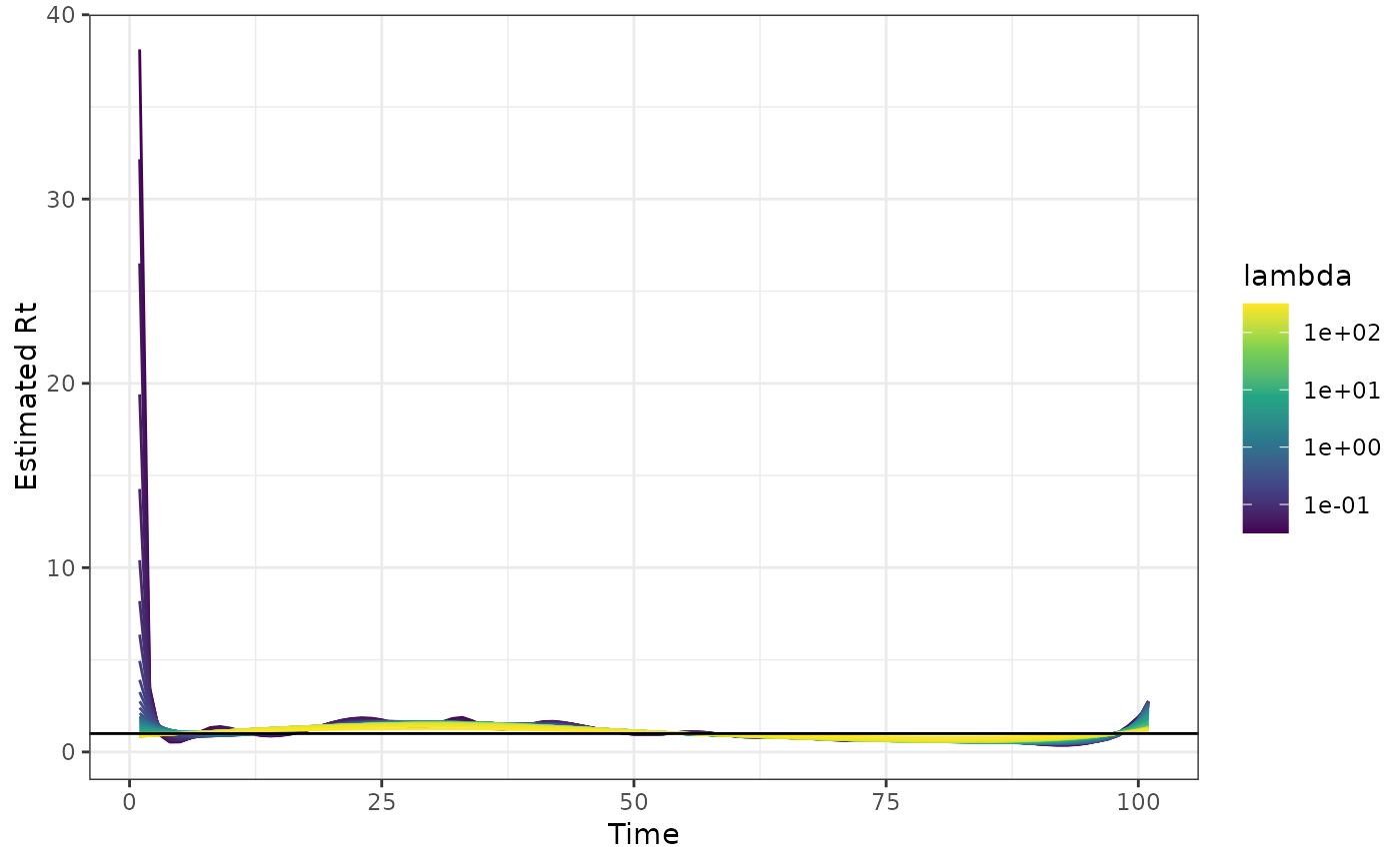
plot(out)


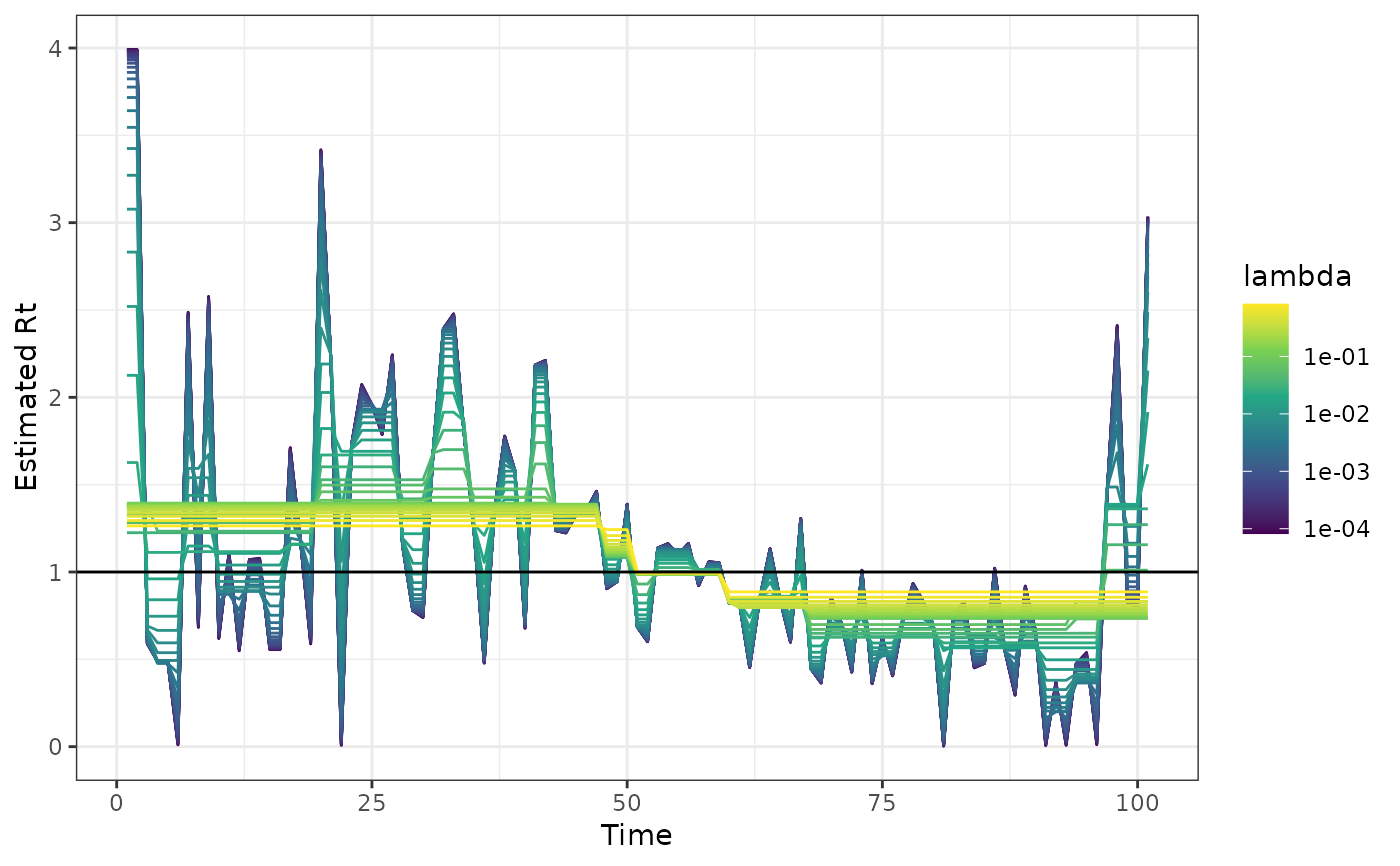
out0 <- estimate_rt(y, korder = 0L, nsol = 40)
out0
#> 
#> Call:  estimate_rt(observed_counts = y, korder = 0L, nsol = 40)
#> 
#> Degree of the estimated piecewise polynomial curve: 0 
#> 
#> Summary of the 40 estimated models:
#> 
#>           lambda index approx_dof niterations
#> Max.    80.25910     1          1           0
#> 3rd Qu.  7.56577    11          9           0
#> Median   0.90318    20         54           0
#> 1st Qu.  0.08514    30         93           0
#> Min.     0.00803    40         96           0
#> 
plot(out0)