Intro to epi forecasting


Daniel J. McDonald

VanML Biostatistics Workshop

23 February 2024
https://dajmcdon.github.io/vanml-epifcast/

Mathematical modelling of disease / epidemics is very old

  • Daniel Bernoulli (1760) - studies inoculation against smallpox

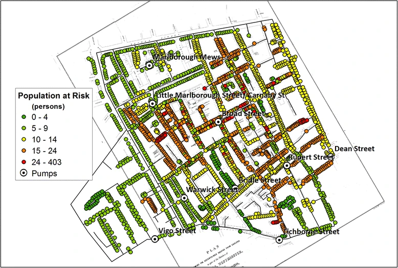
  • John Snow (1855) - cholera epidemic in London tied to a water pump

  • Ronald Ross (1902) - Nobel Prize in Medicine for work on malaria

  • Kermack and McKendrick (1927-1933) - basic epidemic (mathematical) model

Source: Shiode, et al. “The mortality rates and the space-time patterns of John Snow’s cholera epidemic map.” Int J Health Geogr 14, 21 (2015).

Forecasting is also old, but not that old

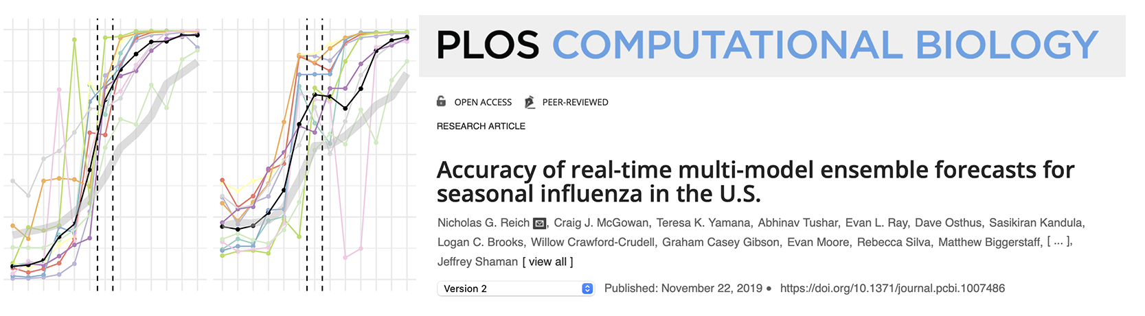
US CDC Flu Challenge began in 2013

CDC’s Influenza Division has collaborated each flu season with external researchers on flu forecasting.
CDC has provided forecasting teams data, relevant public health forecasting targets, and forecast accuracy metrics while teams submit their forecasts, which are based on a variety of methods and data sources, each week.

The Covid-19 Pandemic

  • CDC pivoted their Flu Challenge to Covid-19 in June 2020

  • Similar efforts in Germany and then Europe

  • Nothing similar for Canada

  • CDC now has Flu and Covid simultaneously

Why the Forecast Hubs?

  • Collect public forecasts in a standard format and visualize

  • Used internally by CDC

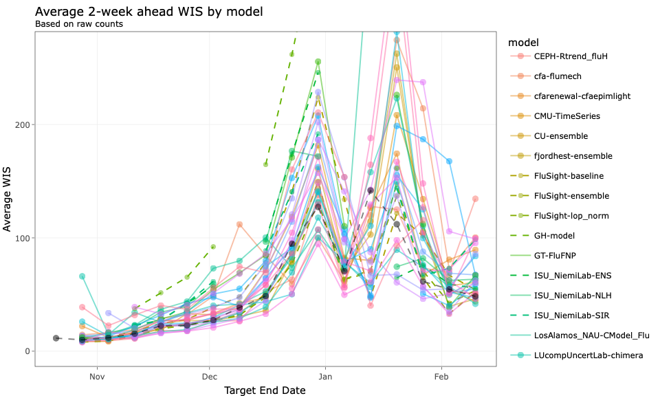
  • Turns out, most individual teams’ forecasts are … not great

  • Combine submissions into an “Ensemble”

https://doi.org/10.1371/journal.pcbi.1007486

Outline

0. History and background

1. Terminology and data

2. Standard forecasting models

3. Building up a Time Series Forecaster

4. Forecast evaluation

5. Hubs and an advertisement

Some terminology

  • As reported on 30 August 2023. Would look different as of 15 April 2023
  • Counts for a Date are updated — “backfill” — as time passes

Revision triangle, Outpatient visits in WA 2022

Data objects

epiprocess::archive_cases_dv_subset$DT |> as_epi_df()
An `epi_df` object, 129,638 x 5 with metadata:
* geo_type  = state
* time_type = day
* as_of     = 2021-12-01

# A tibble: 129,638 × 5
   geo_value time_value version    percent_cli case_rate_7d_av
 * <chr>     <date>     <date>           <dbl>           <dbl>
 1 ca        2020-06-01 2020-06-02       NA               6.63
 2 ca        2020-06-01 2020-06-06        2.14            6.63
 3 ca        2020-06-01 2020-06-07        2.14            6.63
 4 ca        2020-06-01 2020-06-08        2.14            6.63
 5 ca        2020-06-01 2020-06-09        2.11            6.63
 6 ca        2020-06-01 2020-06-10        2.13            6.63
 7 ca        2020-06-01 2020-06-11        2.20            6.63
 8 ca        2020-06-01 2020-06-12        2.23            6.63
 9 ca        2020-06-01 2020-06-13        2.22            6.63
10 ca        2020-06-01 2020-06-14        2.21            6.63
# ℹ 129,628 more rows

Finalized data

  • Counts are revised as time proceeds
  • Want to know the final value
  • Often not available until weeks/months later


Forecasting
At time \(t\), predict the final value for time \(t+h\), \(h > 0\)


Nowcasting
At time \(t\), predict the final value for time \(t\)


Backcasting
At time \(t\), predict the final value for time \(t-h\), \(h < 0\)

Aside on Nowcasting

  • When Epi’s say “nowcasting”, they typically mean “estimate the time-varying instantaneous reproduction number, \(R_t\)

  • My group built {rtestim} doing for this nonparametrically
  • See also {epinow2} and {epinowcast} for flexible (but slow) Bayesian methods based on compartmental models

Mathematical setup

  • Suppose today is time \(t\)

  • Let \(y_i\) denote a series of interest observed at times \(i=1,\ldots, t\).

  • Let \(0< h_1 < \cdots < h_k\) be a collection of forecast horizons.

Our goal

  • Produce point forecasts for the finalized values of \(y_{t+h_1}, \ldots, y_{t+h_k}\).
  • Accompany these with prediction intervals
  • We also have access to \(p\) other time series \(x_{ij},\; i=1,\ldots,t, \; j = 1,\ldots,p\)

  • All may be subject to revisions.

2. Standard forecasting models

Models used for COVID-19 hospitalizations

Quick overview of types

  1. SIR / Compartmental model
  2. Deep Learning / ML
  3. Time series
  • BPagano - SIR
  • CMU - Time Series
  • Colorado (4 versions) - SEIR, different scenarios
  • Georgia Tech - Deep learning…
  • IHME (rarely) - SEIR
  • Johns Hopkins (3 in Applied Physics) - SEIR, Time series, ensemble
  • Johns Hopkins (other, Infection Dynamics) - SEIR
  • Dean Karlen (Physicist at UVic) - Compartmental
  • MOBS-Gleam - Agent based mobility model
  • USC - SEIR
  • UVA - Ensemble of VAR, LSTM, SEIR
  • Prolix - “Offsets obtained by correlations, best linear approximation of reproduction rates (using vaccination approximation) by least euclidean distance, and linear prediction.”

Focus: time series type

Pros:

  • “easy” to implement
  • trivial to incorporate other features (waste water, google searches, auxilliary indicators)
  • massive variety of models and engines (linear models, random forests, boosting, etc.)
  • can be very fast to fit
  • don’t need to know epidemiological parameters (delay distributions, contact rates)
  • pivot to categorical forecasts (classification) or similar
  • can easily borrow information across locations

Cons:

  • doesn’t directly use epi dynamics
  • can’t access things like \(R_t\)
  • no mechanism to interrogate scenarios

Personal hot takes

  • 🐶 Contrast between scenario modelling and forecasting
  • 🐶 You really need to address the revision behaviour
  • 👍 For typical season (influenza) SIR-type gets the dynamics
  • 👎 Novel pathogens make SIR-type extremely difficult
  • 👎 SIR-type requires lots of hand-tuning, and slow to fit
  • 👎 Very difficult for Epi’s at STLTs to implement SIR from scratch
  • 👍 I’m a statistician, so Time Series is much easier for me

Comparison of real-time performance

  • Deep learning isn’t worth it.
  • Hospitalization due to Covid; all US states, weekly, from January 2021 to December 2022

3. Building a time series forecaster

Philosophy of forecasting (general predictive modelling)

We should build up modular components

Be able to add/remove layers of complexity sequentially

  1. Preprocessor: do things to the data before model training
  2. Trainer: train a model on data, resulting in an object
  3. Forecast: make forecasts, using an estimated model object
  4. Postprocessor: do things to the predictions before returning

Examples of preprocessing

EDA type stuff

  1. Making locations commensurate (per capita scaling)
  2. Dealing with revisions (do some nowcasting?)
  3. Detecting and removing outliers
  4. Imputing or removing missing data

Feature engineering

  1. Creating lagged predictors
  2. Day of Week effects
  3. Rolling averages for smoothing (!!!)
  4. Lagged differences
  5. Growth rates instead of raw signals
  6. The sky’s the limit

Calculating growth rates

Outlier detection

Examples of postprocessing

  • Impute missing features
  • Nowcast current values of features
  • Bootstrap to get predictive intervals
  • Invert scaling or other transforms
  • Threshold predictions, [0, max_population]

{epipredict}

https://cmu-delphi.github.io/epipredict

  • Canned forecasters that work out-of-the-box
  • Backtest using the versioned data
  • Easily create features
  • Modify / transform / calibrate forecasts
  • Quickly pivot to new tasks
  • Highly customizable for advanced users

A very specialized plug-in to {tidymodels}

Canned forecasters that work out of the box.

But, you can adjust a lot of options

We currently provide:

  • Baseline flat-line forecaster
  • Autoregressive-type forecaster
  • Autoregressive-type classifier

Canned forecasters that work out of the box.

But, you can adjust a lot of options

Flatline forecaster (CDC Baseline)

For each location, predict \[\hat{y}_{j,\ t+h} = y_{j,\ t}\]

Prediction intervals are determined using the quantiles of the residuals

Canned forecasters that work out of the box.

But, you can adjust a lot of options

AR forecaster

Use an AR model with an extra feature, e.g.: \[\hat{y}_{j,\ t+h} = \mu + a_0 y_{j,\ t} + a_7 y_{j,\ t-7} + b_0 x_{j,\ t} + b_7 x_{j,\ t-7}\]

Here, all predictions (point forecast and intervals) use Quantile Regression

Basic autoregressive forecaster

  • Predict death_rate, 1 week ahead, with 0,7,14 day lags of cases and deaths.
  • Use lm for estimation. Also create intervals.
edf <- case_death_rate_subset # grab some built-in data
canned <- arx_forecaster(
  epi_data = edf, 
  outcome = "death_rate", 
  predictors = c("case_rate", "death_rate")
)

The output is a model object that could be reused in the future, along with the predictions for 7 days from now.

Adjust lots of built-in options

rf <- arx_forecaster(
  epi_data = edf, 
  outcome = "death_rate", 
  predictors = c("case_rate", "death_rate", "fb-survey"),
  trainer = parsnip::rand_forest(mode = "regression"), # use {ranger}
  args_list = arx_args_list(
    ahead = 14, # 2-week horizon
    lags = list(
      case_rate = c(0:4, 7, 14), 
      death_rate = c(0, 7, 14), 
      `fb-survey` = c(0:7, 14)
    ),
    quantile_levels = c(0.01, 0.025, 1:19 / 20, 0.975, 0.99), # 23 ForecastHub quantiles
    quantile_by_key = "geo_value" # vary noise model by location
  )
)

Do (almost) anything manually

# A preprocessing "recipe" that turns raw data into features / response
r <- epi_recipe(edf) |>
  step_epi_lag(case_rate, lag = c(0, 1, 2, 3, 7, 14)) |>
  step_epi_lag(death_rate, lag = c(0, 7, 14)) |>
  step_epi_ahead(death_rate, ahead = 14) |>
  step_epi_naomit()

# A postprocessing routine describing what to do to the predictions
f <- frosting() |>
  layer_predict() |>
  layer_threshold(.pred, lower = 0) |> # predictions / intervals should be non-negative
  layer_add_target_date() |>
  layer_add_forecast_date()

# Bundle up the preprocessor, training engine, and postprocessor
# We use quantile regression
ewf <- epi_workflow(r, quantile_reg(quantile_levels = c(.1, .5, .9)), f)

# Fit it to data (we could fit this to ANY data that has the same format)
trained_ewf <- ewf |> fit(edf)

# examines the recipe to determine what we need to make the prediction
latest <- get_test_data(r, edf)

# we could make predictions using the same model on ANY test data
preds <- trained_ewf |> predict(new_data = latest)

Visualize a result for 1 forecast date, 2 locations

Code
edf <- case_death_rate_subset
fd <- as.Date("2021-11-30")
geos <- c("wa", "ca")
h <- 1:28

tedf <- edf |> filter(time_value >= fd)
# use most recent 3 months for training
edf <- edf |> filter(time_value < fd, time_value >= fd - 90L)

rec <- epi_recipe(edf) |>
  step_epi_lag(case_rate, lag = c(0, 7, 14, 21)) |>
  step_epi_lag(death_rate, lag = c(0, 7, 14)) |>
  step_epi_ahead(death_rate, ahead = h)

f <- frosting() |>
  layer_predict() |>
  layer_unnest(.pred) |>
  layer_naomit(distn) |>
  layer_add_forecast_date() |>
  layer_threshold(distn)

ee <- smooth_quantile_reg(
  quantile_levels = c(.05, .1, .25, .5, .75, .9, .95), outcome_locations = h
)

ewf <- epi_workflow(rec, ee, f)
  
the_fit <- ewf |> fit(edf)

latest <- get_test_data(rec, edf, fill_locf = TRUE) |> 
  filter(geo_value %in% geos)

preds <- predict(the_fit, new_data = latest) |>
  mutate(forecast_date = fd, target_date = fd + ahead) |>
  select(geo_value, target_date, .pred_distn = distn) |>
  mutate(.pred = median(.pred_distn))
  
ggplot(preds) |>
  plot_bands(preds, fill = tertiary) +
  geom_vline(xintercept = ymd("2021-11-30"), linetype = "dashed") +
  geom_line(
    data = case_death_rate_subset |> 
      filter(time_value > ymd("2021-09-30"), geo_value %in% geos),
    mapping = aes(x = time_value, y = death_rate)) +
  geom_line(
    mapping = aes(x = target_date, y = .pred), colour = primary,
    linewidth = 1.5) +
  facet_wrap(~geo_value) +
  ylab("Covid deaths per 100K population") + xlab("Date") +
  scale_y_continuous(expand = expansion(), limits = c(0, .75))

4. Evaluating forecasts

Community standard forecast format, FluSight Ensemble

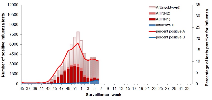
  • Choose a target signal, relevant to PH, incident hospitalizations
  • Usually submit (every week), for weekly or daily horizons, up to a month out
  • Point forecast and a set of quantiles c(0.01, 0.025, 1:19 / 20, 0.975, 0.99)
  • Could produce categorical forecasts (“way up”, “up”, “steady”, “down”)
  • Historically, could submit samples from a distribution

Headline “score”

Weighted Interval Score (Bracher et al., 2021)

\[ \textrm{WIS}(F, Y) = \sum_{\alpha} \big\{\alpha(u_\alpha - \ell_\alpha) + 2 \cdot \textrm{dist} (Y,\ [\ell_\alpha,\ u_\alpha])\big\} \]

  • Calculated for each target (forecast date, location, horizon)

  • For each Interval:

    1. Width of interval.
    2. Under prediction (AE to the top)
    3. Over prediction (AE to the bottom)
  • Weighted average using probability content

  • Mathematically equivalent to an average of quantile losses

  • Discrete approximation of CRPS

  • Figures from http://reichlab.io/flusight-eval/

FluSight 2 week WIS

Overprediction and underprediction
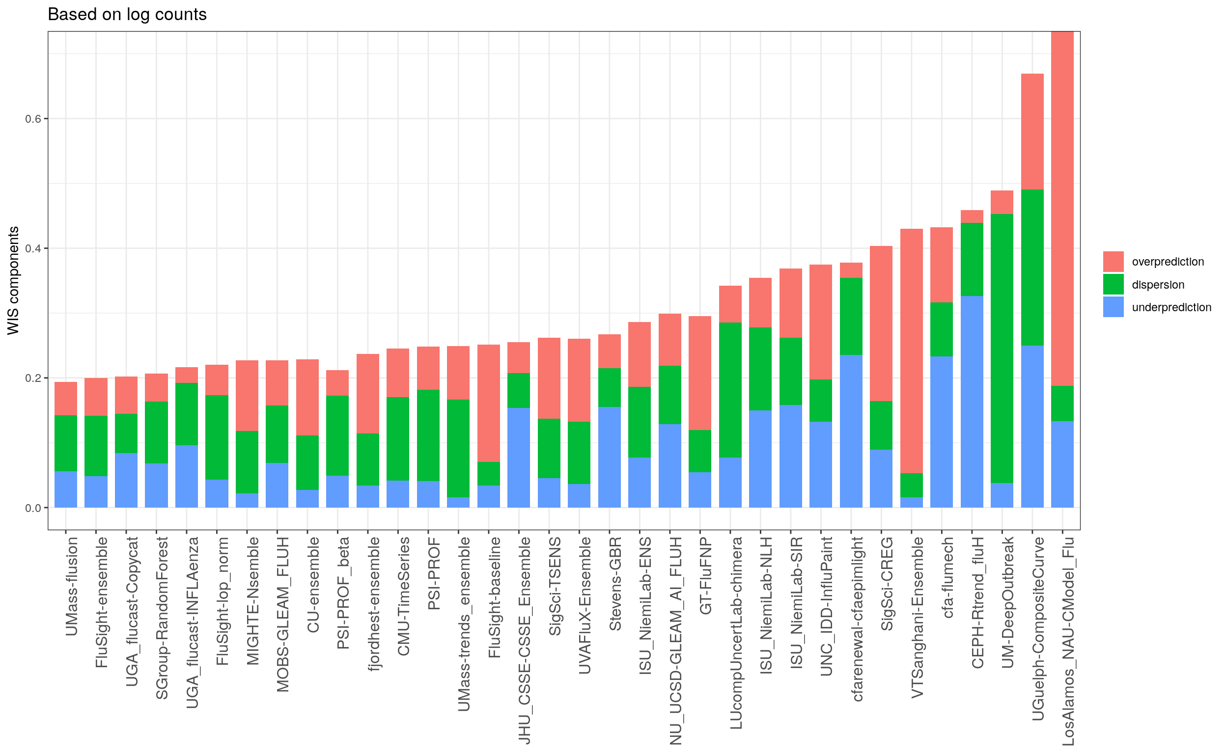
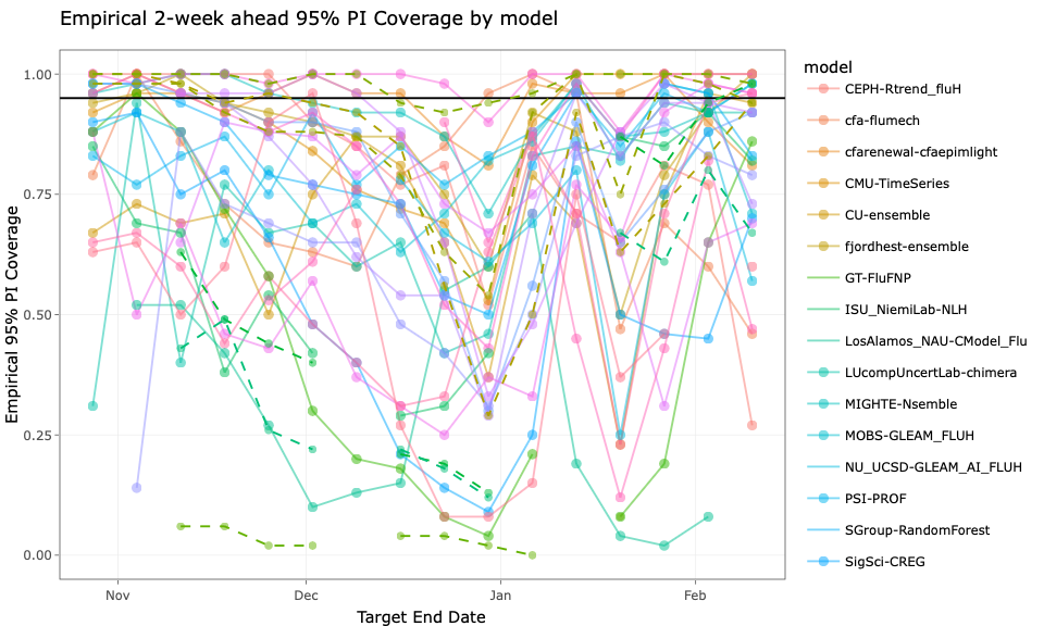
Calibration

Comparing across disparate targets

  • Target = (forecast date, horizon, location)
  • Everything so far is “per target”
  • Better (in my view), to normalize by “difficulty”
  • Forecasters that do well when it’s “easy” aren’t adding anything
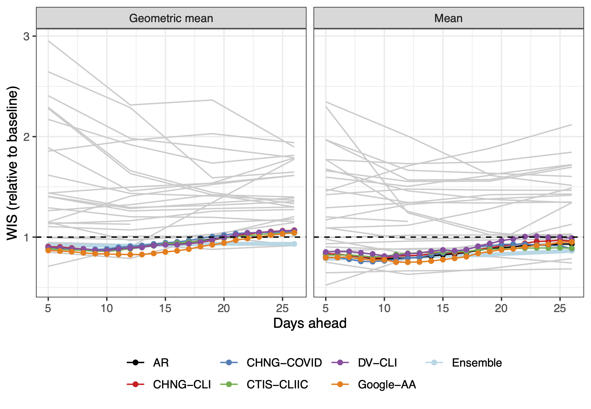
5. Hubs and an advertisement

Forecast Hubs

Current

  • The US CDC runs
    • the FluSight Modelling Hub
    • RSV Hub (just started)
  • RespiCast - European CDC
  • CDPH - West Nile Virus (coming in May)
  • CFA runs Covid Hub (US)
  • CFA starting an Rt Hub?

Past

  • Scenario Modelling Hub (US) for Covid
  • German Flu Hospitalization Hub
  • European Covid Hub
  • Germany + Poland Covid Hub

Why the hubs?

  • Encourage standard data formats
  • Provide forecasts to public health
  • Create Ensembles of participating teams with much better performance
  • Create communities of forecasters

Goal: Create a Hub for Canada to begin in September

  • Need target data
  • Need teams to participate

Target data?

FluWatch Weekly Reports

  • Format is ick.
  • We’ll try to make this available.
  • And it’s history.
  • Some is versioned

So you’re going to participate?!

Some suggestions for any type of forecasting

  1. Be cognizant of backfill
  2. Correct outliers / anomalies
  3. Combine across locations (probably internationally as well)
  4. Incorporate curated auxilliary signals (throwing in everything isn’t great)
  5. To produce weekly forecasts, train on trailing 7-day averages (7x the data)
  6. Use quantile regression or nonparametric prediction intervals
  7. Examine your forecasts!
  8. Regularly evaluate performance

Thanks

  • The CMU Delphi Team
  • Centers for Disease Control and Prevention.
  • Council of State and Territorial Epidemiologists
  • NSERC
  • Optum/United Healthcare, Change Healthcare.
  • Google, Facebook, Amazon Web Services.
  • Quidel, SafeGraph, Qualtrics.