Plot solution paths from a sparsegl object.

Produces a coefficient profile plot of a fitted sparsegl() object. The result is a ggplot2::ggplot(). Additional user modifications can be added as desired.

Usage

# S3 method for sparsegl
plot(
  x,
  y_axis = c("coef", "group"),
  x_axis = c("lambda", "penalty"),
  add_legend = n_legend_values < 20,
  ...
)

Arguments

x

Fitted "sparsegl" object, produced by sparsegl().

y_axis

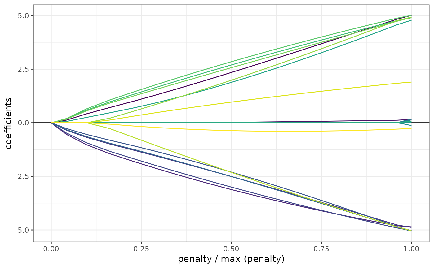
Variable on the y_axis. Either the coefficients (default) or the group norm.

x_axis

Variable on the x-axis. Either the (log)-lambda sequence (default) or the value of the penalty. In the second case, the penalty is scaled by its maximum along the path.

add_legend

Show the legend. Often, with many groups/predictors, this can become overwhelming. The default produces a legend if the number of groups/predictors is less than 20.

...

Not used.

See also

sparsegl().

Examples

n <- 100
p <- 20
X <- matrix(rnorm(n * p), nrow = n)
eps <- rnorm(n)
beta_star <- c(rep(5, 5), c(5, -5, 2, 0, 0), rep(-5, 5), rep(0, (p - 15)))
y <- X %*% beta_star + eps
groups <- rep(1:(p / 5), each = 5)
fit1 <- sparsegl(X, y, group = groups)
plot(fit1, y_axis = "coef", x_axis = "penalty")