Getting started with sparsegl

This package provides tools for fitting regularization paths for sparse group-lasso penalized learning problems. The model is fit for a sequence of the regularization parameters.

The strengths and improvements that this package offers relative to other sparse group-lasso packages are as follows:

Compiled Fortran code significantly speeds up the sparse group-lasso estimation process.
So-called “strong rules” are implemented during group wise coordinate descent steps screen out groups which are likely to be 0 at the solution.
The design matrix X may be a sparse.
An estimate_risk() function may be used to evaluate the quality of fitted models via information criteria, providing a means for model selection if cross-validation is too computationally costly.
Additional exponential families may be fit (though this is typically slower).

For additional details, see Liang, Cohen, Sólon Heinsfeld, Pestilli, and McDonald (2024).

Installing

You can install the released version of sparsegl from CRAN with:

install.packages("sparsegl")

You can install the development version from GitHub with:

# install.packages("remotes")
remotes::install_github("dajmcdon/sparsegl")

Vignettes are not included in the package by default. If you want to include vignettes, then use this modified command:

remotes::install_github(
  "dajmcdon/sparsegl",
  build_vignettes = TRUE, 
  dependencies = TRUE
)

For this getting-started vignette, first, we will randomly generate X, an input matrix of predictors of dimension $n\times p$ . To create y, a real-valued vector, we use either a

Linear Regression model: $y = X\beta^* + \epsilon$ .
Logistic regression model: $y = (y_1, y_2, \cdots, y_n)$ , where $y_i \sim \text{Bernoulli}\left(\frac{1}{1 + \exp(-x_i^\top \beta^*)}\right)$ , $i = 1, 2, \cdots, n.$

where the coefficient vector $\beta^*$ is specified as below, and the white noise $\epsilon$ follows a standard normal distribution. Then the sparse group-lasso problem is formulated as the sum of mean squared error (linear regression) or logistic loss (logistic regression) and a convex combination of the $\ell_1$ lasso penalty with an $\ell_2$ group lasso penalty:

Linear regression: $\min_{\beta\in\mathbb{R}^p}\left(\frac{1}{2n} \rVert y - \sum_g X^{(g)}\beta^{(g)}\rVert_2^2 + (1-\alpha)\lambda\sum_g \sqrt{|g|}\rVert\beta^{(g)}\rVert_2 + \alpha\lambda\rVert\beta\rVert_1 \right) \qquad (*).$
Logistic regression: $\min_{\beta\in\mathbb{R}^p}\left(\frac{1}{2n}\sum_{i=1}^n \log\left(1 + \exp\left(-y_ix_i^\top\beta\right)\right) + (1-\alpha)\lambda\sum_g \sqrt{|g|}\rVert\beta^{(g)}\rVert_2 + \alpha\lambda\rVert\beta\rVert_1 \right) \qquad (**).$

where

$X^{(g)}$ is the submatrix of $X$ with columns corresponding to the features in group $g$ .
$\beta^{(g)}$ is the corresponding coefficients of the features in group $g$ .
$|g|$ is the number of predictors in group $g$ .
$\alpha$ adjusts the weight between lasso penalty and group-lasso penalty.
$\lambda$ fine-tunes the size of penalty imposed on the model to control the number of nonzero coefficients.

library(sparsegl)
set.seed(1010)
n <- 100
p <- 200
X <- matrix(data = rnorm(n * p, mean = 0, sd = 1), nrow = n, ncol = p)
beta_star <- c(
  rep(5, 5), c(5, -5, 2, 0, 0), rep(-5, 5),
  c(2, -3, 8, 0, 0), rep(0, (p - 20))
)
groups <- rep(1:(p / 5), each = 5)

# Linear regression model
eps <- rnorm(n, mean = 0, sd = 1)
y <- X %*% beta_star + eps

# Logistic regression model
pr <- 1 / (1 + exp(-X %*% beta_star))
y_binary <- rbinom(n, 1, pr)

`sparsegl()`

Given an input matrix X, and a response vector y, a sparse group-lasso regularized linear model is estimated for a sequence of penalty parameter values. The penalty is composed of lasso penalty and group lasso penalty. The other main arguments the users might supply are:

group: a vector with consecutive integers of length p indicating the grouping of the features. By default, each group only contains one feature if without initialization.
family: A character string specifying the likelihood to use, could be either linear regression "gaussian" or logistic regression loss "binomial". Default is "gaussian". If other exponential families are required, a stats::family() object may be used (e.g. poisson()). In that case, arguments providing observation weights or offset terms are allowed as well.
pf_group: Separate penalty weights can be applied to each group $\beta_g$ to allow differential shrinkage. Can be 0 for some groups, which implies no shrinkage. The default value for each entry is the square-root of the corresponding size of each group.
pf_sparse: Penalty factor on $\ell_1$ -norm, a vector the same length as the total number of columns in x. Each value corresponds to one predictor Can be 0 for some predictors, which implies that predictor will be receive only the group penalty.
asparse: changes the weight of lasso penalty, referring to $\alpha$ in $(*)$ and $(**)$ above: asparse = $1$ gives the lasso penalty only. asparse = $0$ gives the group lasso penalty only. The default value of asparse is $0.05$ .
lower_bnd: lower bound for coefficient values, a vector in length of 1 or the number of groups including non-positive numbers only. Default value for each entry is - $\infty$ .
upper_bnd: upper bound for coefficient values, a vector in length of 1 or the number of groups including non-negative numbers only. Default value for each entry is $\infty$ .

fit1 <- sparsegl(X, y, group = groups)

Plotting `sparsegl` objects

This function displays nonzero coefficient curves for each penalty parameter lambda values in the regularization path for a fitted sparsegl object. The arguments of this function are:

y_axis: can be set with either "coef" or "group". Default is "coef".
x_axis: can be set with either "lambda" or "penalty". Default is "lambda".

To elaborate on these arguments:

The plot with y_axis = "group" shows the group norms against the log-lambda or the scaled group norm vector. Each group norm is defined by: $\alpha\rVert\beta^{(g)}\rVert_1 + (1 - \alpha)\sum_g\rVert\beta^{(g)}\rVert_2$ Curves are plotted in the same color if the corresponding features are in the same group. Note that the number of curves shown on the plots may be less than the actual number of groups since only the groups containing nonzero features for at least one $\lambda$ in the sequence are included.
The plot with y_axis = "coef" shows the estimated coefficients against the lambda or the scaled group norm. Again, only the features with nonzero estimates for at least one $\lambda$ value in the sequence are displayed.
The plot with x_axis = "lambda" indicates the x_axis displays $\log(\lambda)$ .
The plot with x_axis = "penalty" indicates the x_axis displays the scaled group norm vector. Each element in this vector is defined by: $\frac{\alpha\rVert \beta\rVert_1 + (1-\alpha)\sum_g\rVert \beta^{(g)}\rVert_2}{\max_\beta\left(\alpha \rVert \beta\rVert_1 + (1-\alpha)\sum_g\rVert \beta^{(g)}\rVert_2\right)}$

plot(fit1, y_axis = "group", x_axis = "lambda")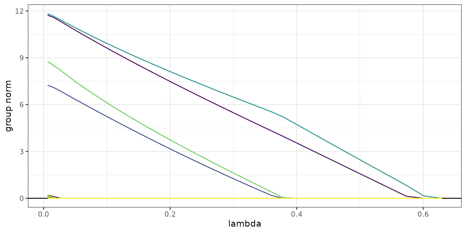

plot(fit1, y_axis = "coef", x_axis = "penalty", add_legend = FALSE)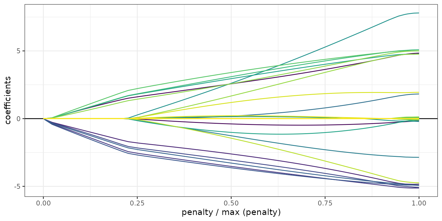

`cv.sparsegl()`

This function performs k-fold cross-validation (cv). It takes the same arguments X, y, group, which are specified above, with additional argument pred.loss for the error measure. Options are "default", "mse", "deviance", "mae", and "misclass". With family = "gaussian", "default" is equivalent to "mse" and "deviance". In general, "deviance" will give the negative log-likelihood. The option "misclass" is only available if family = "binomial".

fit_l1 <- cv.sparsegl(X, y, group = groups, pred.loss = "mae")
plot(fit_l1)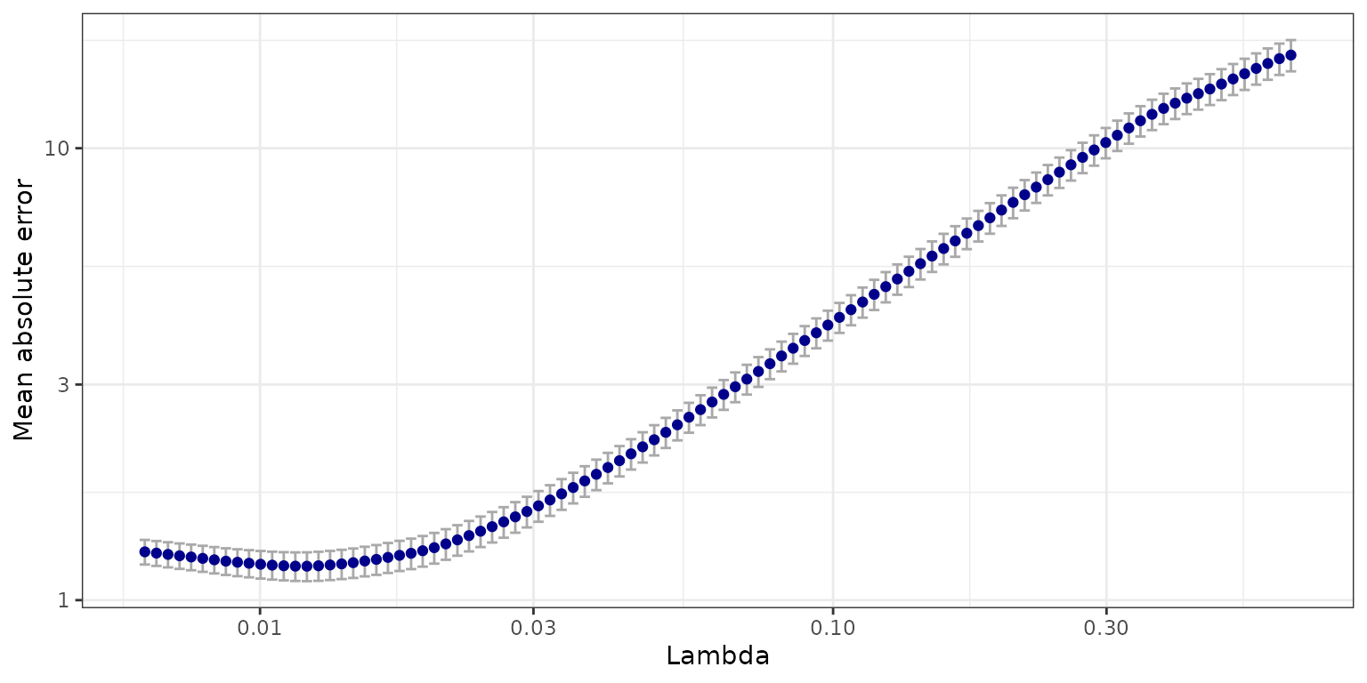

Methods

A number of S3 methods are provided for both sparsegl and cv.sparsegl objects.

coef() and predict() return a matrix of coefficients and predictions $\hat{y}$ given a matrix X at each lambda respectively. The optional s argument may provide a specific value of $\lambda$ (not necessarily part of the original sequence), or, in the case of a cv.sparsegl object, a string specifying either "lambda.min" or "lambda.1se".

coef <- coef(fit1, s = c(0.02, 0.03))
predict(fit1, newx = X[100, ], s = fit1$lambda[2:3])
#>             s1        s2
#> [1,] -4.071804 -4.091689
predict(fit_l1, newx = X[100, ], s = "lambda.1se")
#>             s1
#> [1,] -15.64857
print(fit1)
#> 
#> Call:  sparsegl(x = X, y = y, group = groups) 
#> 
#> Summary of Lambda sequence:
#>          lambda index nnzero active_grps
#> Max.    0.62948     1      0           0
#> 3rd Qu. 0.19676    26     20           4
#> Median  0.06443    50     19           4
#> 1st Qu. 0.02014    75     25           5
#> Min.    0.00629   100    111          23

`estimate_risk()`

With extremely large data sets, cross validation may be to slow for tuning parameter selection. This function uses the degrees of freedom to calculate various information criteria. This function uses the “unknown variance” version of the likelihood. Only implemented for Gaussian regression. The constant is ignored (as in stats::extractAIC()).

object: a fitted sparsegl object.
type: three types of penalty used for calculation:
- AIC (Akaike information criterion): $2 df / n$
- BIC (Bayesian information criterion): $2 df\log(n) / n$
- GCV (Generalized cross validation): $-2\log(1 - df / n)$

where df is the degree-of-freedom, and n is the sample size.

approx_df: indicates if an approximation to the correct degree-of-freedom at each penalty parameter $\lambda$ should used. Default is FALSE and the program will compute an unbiased estimate of the exact degree-of-freedom.

The df component of a sparsegl object is an approximation (albeit a fairly accurate one) to the actual degrees-of-freedom. However, computing the exact value requires inverting a portion of $\mathbf{X}^\top \mathbf{X}$ . So this computation may take some time (the default computes the exact df). For more details about how this formula, see Vaiter, Deledalle, Peyré, et al., (2012).

risk <- estimate_risk(fit1, X, approx_df = FALSE)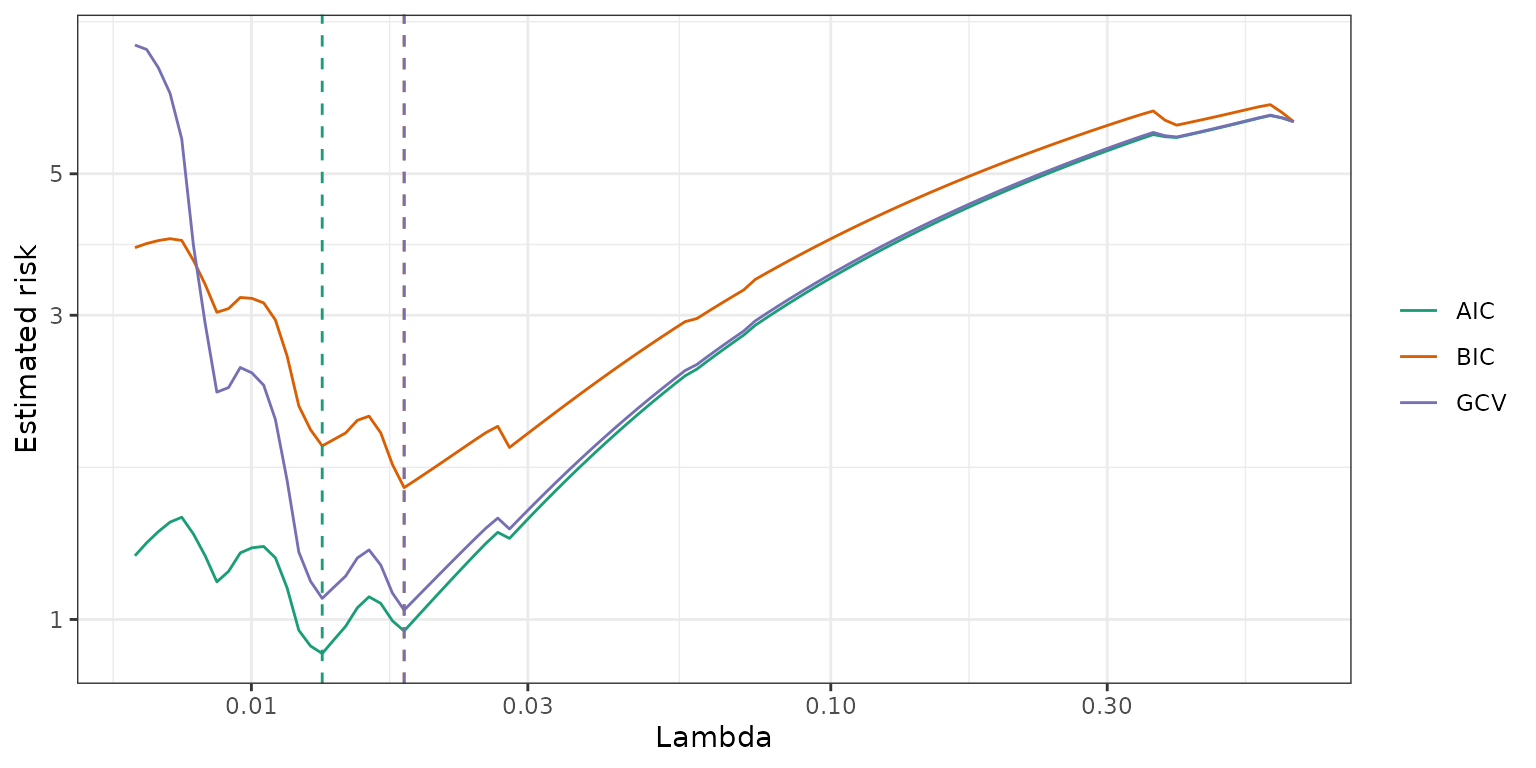

References

Liang, X., Cohen, A., Sólon Heinsfeld, A., Pestilli, F., and McDonald, D.J. 2024. “sparsegl: An R Package for Estimating Sparse Group Lasso.” Journal of Statistical Software 110(6), 1–23. https://doi.org/10.18637/jss.v110.i06.

Vaiter S, Deledalle C, Peyré G, Fadili J, and Dossal C. 2012. “The Degrees of Freedom of the Group Lasso for a General Design.” https://arxiv.org/abs/1212.6478.

Installing

sparsegl()

Plotting sparsegl objects