3 Examples of Preprocessing and Models
3.1 Introduction
The epipredict package utilizes the tidymodels framework, namely
{recipes} for
dplyr-like pipeable sequences
of feature engineering and {parsnip} for a
unified interface to a range of models.
epipredict has additional customized feature engineering and preprocessing
steps, such as step_epi_lag(), step_population_scaling(),
step_epi_naomit(). They can be used along with
steps from the recipes package for more feature engineering.
In this vignette, we will illustrate some examples of how to use epipredict
with recipes and parsnip for different purposes of epidemiological forecasting.
We will focus on basic autoregressive models, in which COVID cases and
deaths in the near future are predicted using a linear combination of cases and
deaths in the near past.
The remaining vignette will be split into three sections. The first section, we will use a Poisson regression to predict death counts. In the second section, we will use a linear regression to predict death rates. Last but not least, we will create a classification model for hotspot predictions.
3.2 Poisson Regression
During COVID-19, the U.S. Centers for Disease Control and Prevention (CDC) collected models and forecasts to characterize the state of an outbreak and its course. They use it to inform public health decision makers on potential consequences of deploying control measures.
One of the outcomes that the CDC forecasts is death counts from COVID-19.
Although there are many state-of-the-art models, we choose to use Poisson
regression, the textbook example for modeling count data, as an illustration
for using the epipredict package with other existing tidymodels packages.
geos <- c("ca", "fl", "tx", "ny", "nj")
x <- covidcast(
  data_source = "jhu-csse",
  signals = "confirmed_incidence_num",
  time_type = "day",
  geo_type = "state",
  time_values = epirange(20210604, 20211231),
  geo_values = geos) %>%
  fetch_tbl() %>%
  select(geo_value, time_value, cases = value)

y <- covidcast(
  data_source = "jhu-csse",
  signals = "deaths_incidence_num",
  time_type = "day",
  geo_type = "state",
  time_values = epirange(20210604, 20211231),
  geo_values = geos) %>%
  fetch_tbl() %>%
  select(geo_value, time_value, deaths = value)

counts_subset <- full_join(x, y, by = c("geo_value", "time_value")) %>%
  as_epi_df()
The counts_subset dataset comes from the epidatr package, and
contains the number of confirmed cases and deaths from June 4, 2021 to
Dec 31, 2021 in some U.S. states.
We wish to predict the 7-day ahead death counts with lagged cases and deaths. Furthermore, we will let each state be a dummy variable. Using differential intercept coefficients, we can allow for an intercept shift between states.
One possible model takes the form \[\begin{aligned} \log\left( \mu_{t+7} \right) &{}= \beta_0 + \delta_1 s_{\text{state}_1} + \delta_2 s_{\text{state}_2} + \cdots + \nonumber \\ &\quad\beta_1 \text{deaths}_{t} + \beta_2 \text{deaths}_{t-7} + \beta_3 \text{cases}_{t} + \beta_4 \text{cases}_{t-7}, \end{aligned}\]where \(\mu_{t+7} = \mathbb{E}(\text{deaths}_{t+7})\), and \(\text{deaths}_{t+7}\) is assumed to follow a Poisson distribution with mean \(\mu_{t+7}\); \(s_{\text{state}}\) are dummy variables for each state and take values of either 0 or 1.
Preprocessing steps will be performed to prepare the
data for model fitting. But before diving into them, it will be helpful to understand what roles are in the recipes framework.
Aside on recipes
recipes can assign one or more roles to each column in the data. The roles
are not restricted to a predefined set; they can be anything.
For most conventional situations, they are typically “predictor” and/or
“outcome.” Additional roles enable targeted step_*() operations on specific
variables or groups of variables.
In our case, the role predictor is given to explanatory variables on the
right-hand side of the model (in the equation above).
The role outcome is the response variable
that we wish to predict. geo_value and time_value are predefined roles
that are unique to the epipredict package. Since we work with epi_df
objects, all datasets should have geo_value and time_value passed through
automatically with these two roles assigned to the appropriate columns in the data.
The recipes package also allows manual alterations of roles
in bulk. There are a few handy functions that can be used together to help us
manipulate variable roles easily.
update_role()alters an existing role in the recipe or assigns an initial role to variables that do not yet have a declared role.
add_role()adds an additional role to variables that already have a role in the recipe, without overwriting old roles.
remove_role()eliminates a single existing role in the recipe.
End aside
Notice in the following preprocessing steps, we used add_role() on
geo_value_factor since, currently, the default role for it is raw, but
we would like to reuse this variable as a predictor.
counts_subset <- counts_subset %>%
  mutate(geo_value_factor = as.factor(geo_value)) %>%
  as_epi_df()

epi_recipe(counts_subset)

r <- epi_recipe(counts_subset) %>%
  add_role(geo_value_factor, new_role = "predictor") %>%
  step_dummy(geo_value_factor) %>%
  ## Occasionally, data reporting errors / corrections result in negative
  ## cases / deaths
  step_mutate(cases = pmax(cases, 0), deaths = pmax(deaths, 0)) %>%
  step_epi_lag(cases, deaths, lag = c(0, 7)) %>%
  step_epi_ahead(deaths, ahead = 7, role = "outcome") %>%
  step_epi_naomit()
After specifying the preprocessing steps, we will use the parsnip package for
modeling and producing the prediction for death count, 7 days after the
latest available date in the dataset.
latest <- get_test_data(r, counts_subset)

wf <- epi_workflow(r, parsnip::poisson_reg()) %>%
  fit(counts_subset)

predict(wf, latest) %>% filter(!is.na(.pred))
#> An `epi_df` object, 5 x 3 with metadata:
#> * geo_type  = state
#> * time_type = day
#> * as_of     = 2023-04-04 16:26:23
#>
#> # A tibble: 5 × 3
#>   geo_value time_value .pred
#> * <chr>     <date>     <dbl>
#> 1 ca        2021-12-31 108.
#> 2 fl        2021-12-31 270.
#> 3 nj        2021-12-31  22.5
#> 4 ny        2021-12-31  94.8
#> 5 tx        2021-12-31  91.0
Note that the time_value corresponds to the last available date in the
training set, NOT to the target date of the forecast
(2022-01-07).
Let’s take a look at the fit:
extract_fit_engine(wf)
#>
#> Call:  stats::glm(formula = ..y ~ ., family = stats::poisson, data = data)
#>
#> Coefficients:
#>         (Intercept)  geo_value_factor_fl
#>           3.970e+00           -1.487e-01
#> geo_value_factor_nj  geo_value_factor_ny
#>          -1.425e+00           -6.865e-01
#> geo_value_factor_tx          lag_0_cases
#>           3.025e-01            1.339e-05
#>         lag_7_cases         lag_0_deaths
#>           1.717e-06            1.731e-03
#>        lag_7_deaths
#>           8.566e-04
#>
#> Degrees of Freedom: 984 Total (i.e. Null);  976 Residual
#> Null Deviance:       139600
#> Residual Deviance: 58110     AIC: 62710
Alternative forms of Poisson regression or particular computational approaches
can be applied via arguments to parsnip::poisson_reg() for some common
settings, and by using parsnip::set_engine() to use a specific Poisson
regression engine and to provide additional engine-specific customization.
3.3 Linear Regression
For COVID-19, the CDC required submission of case and death count predictions.
However, the Delphi Group preferred to train on rate data instead, because it
puts different locations on a similar scale (eliminating the need for location-specific intercepts).
We can use a linear regression to predict the death rates and use state
population data to scale the rates to counts.3 We will do so using
layer_population_scaling() from the epipredict package. (We could also use
step_population_scaling() from the epipredict package to prepare rate data
from count data in the preprocessing recipe.)
Additionally, when forecasts are submitted, prediction intervals should be
provided along with the point estimates. This can be obtained via postprocessing
using
layer_residual_quantiles(). It is worth pointing out, however, that
layer_residual_quantiles() should be used before population scaling or else
the transformation will make the results uninterpretable.
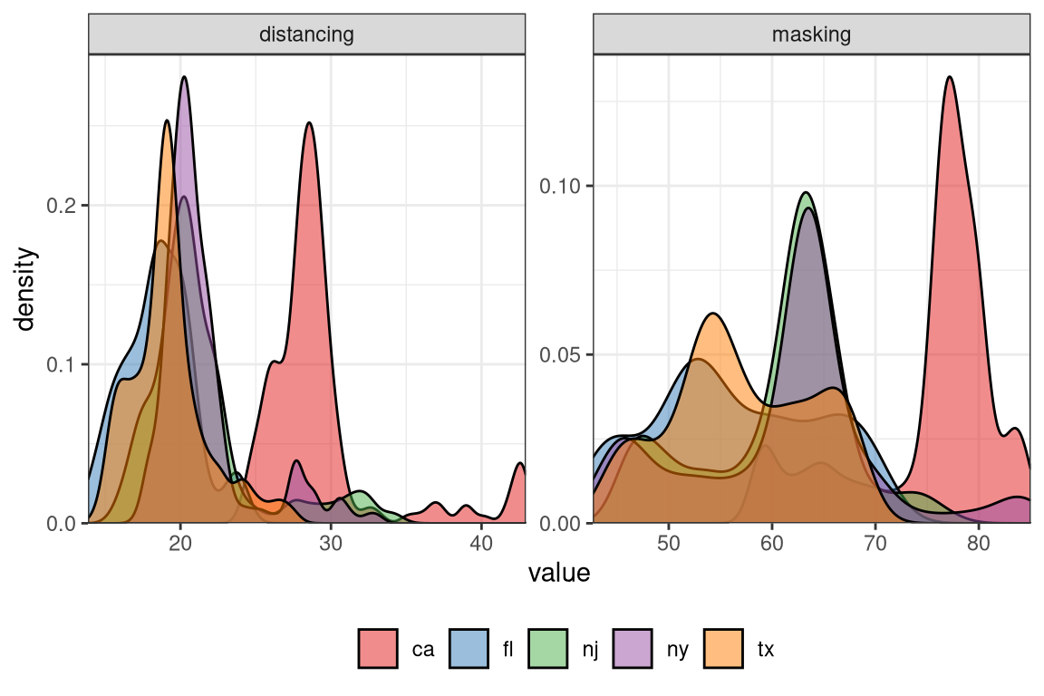
We wish, now, to predict the 7-day ahead death counts with lagged case rates and death rates, along with some extra behaviourial predictors. Namely, we will use survey data from COVID-19 Trends and Impact Survey.
The survey data provides the estimated percentage of people who wore a mask for most or all of the time while in public in the past 7 days and the estimated percentage of respondents who reported that all or most people they encountered in public in the past 7 days maintained a distance of at least 6 feet.
State-wise population data from the 2019 U.S. Census is included in this package
and will be used in layer_population_scaling().
behav_ind_mask <- covidcast(
  data_source = "fb-survey",
  signals = "smoothed_wwearing_mask_7d",
  time_type = "day",
  geo_type = "state",
  time_values = epirange(20210604, 20211231),
  geo_values = geos)  %>%
  fetch_tbl() %>%
  select(geo_value, time_value, masking = value)

behav_ind_distancing <- covidcast(
  data_source = "fb-survey",
  signals = "smoothed_wothers_distanced_public",
  time_type = "day",
  geo_type = "state",
  time_values = epirange(20210604, 20211231),
  geo_values = geos)  %>%
  fetch_tbl() %>%
  select(geo_value, time_value, distancing = value)

pop_dat <- state_census %>% select(abbr, pop)

behav_ind <- behav_ind_mask %>%
  full_join(behav_ind_distancing, by = c("geo_value", "time_value"))
Rather than using raw mask-wearing / social-distancing metrics, for the sake of illustration, we’ll convert both into categorical predictors.
We will take a subset of death rate and case rate data from the built-in dataset
case_death_rate_subset.
jhu <- filter(
  case_death_rate_subset,
  time_value >= "2021-06-04",
  time_value <= "2021-12-31",
  geo_value %in% c("ca","fl","tx","ny","nj")
)
Preprocessing steps will again rely on functions from the epipredict package as well
as the recipes package.
There are also many functions in the recipes package that allow for
scalar transformations,
such as log transformations and data centering. In our case, we will
center the numerical predictors to allow for a more meaningful interpretation of the
intercept.
jhu <- jhu %>%
  mutate(geo_value_factor = as.factor(geo_value)) %>%
  left_join(behav_ind, by = c("geo_value", "time_value")) %>%
  as_epi_df()

r <- epi_recipe(jhu) %>%
  add_role(geo_value_factor, new_role = "predictor") %>%
  step_dummy(geo_value_factor) %>%
  step_epi_lag(case_rate, death_rate, lag = c(0, 7, 14)) %>%
  step_mutate(masking = cut_number(masking, 5),
              distancing = cut_number(distancing, 5)) %>%
  step_epi_ahead(death_rate, ahead = 7, role = "outcome") %>%
  step_center(contains("lag"), role = "predictor") %>%
  step_epi_naomit()
As a sanity check we can examine the structure of the training data:
glimpse(slice_sample(bake(prep(r, jhu), jhu), n = 6))
#> Rows: 6
#> Columns: 17
#> $ time_value          <date> 2021-07-22, 2021-07-25, 2021-…
#> $ geo_value           <chr> "tx", "ny", "ca", "ca", "fl", …
#> $ case_rate           <dbl> 14.282426, 6.909115, 9.655756,…
#> $ death_rate          <dbl> 0.0836880, 0.0273350, 0.201758…
#> $ masking             <fct> "[42.7,52.8]", "[42.7,52.8]", …
#> $ distancing          <fct> "(18.4,19.8]", "(18.4,19.8]", …
#> $ geo_value_factor_fl <dbl> 0, 0, 0, 0, 1, 0
#> $ geo_value_factor_nj <dbl> 0, 0, 0, 0, 0, 0
#> $ geo_value_factor_ny <dbl> 0, 1, 0, 0, 0, 1
#> $ geo_value_factor_tx <dbl> 1, 0, 0, 0, 0, 0
#> $ lag_0_case_rate     <dbl> -12.65924, -20.03255, -17.2859…
#> $ lag_7_case_rate     <dbl> -18.420571, -22.365630, -12.43…
#> $ lag_14_case_rate    <dbl> -21.587091, -24.008687, -13.60…
#> $ lag_0_death_rate    <dbl> -0.1981856, -0.2545386, -0.080…
#> $ lag_7_death_rate    <dbl> -0.1865082, -0.2523222, -0.068…
#> $ lag_14_death_rate   <dbl> -0.2054840, -0.2567549, -0.065…
#> $ ahead_7_death_rate  <dbl> 0.1221261, 0.0347229, 0.206839…
Before directly predicting the results, we need to add postprocessing layers to
obtain the death counts instead of death rates. Note that the rates used so
far are “per 100K people” rather than “per person.” We’ll also use quantile
regression with the quantile_reg engine rather than ordinary least squares
to create median predictions and a 90% prediction interval.
f <- frosting() %>%
  layer_predict() %>%
  layer_add_target_date("2022-01-07") %>%
  layer_threshold(.pred, lower = 0) %>%
  layer_quantile_distn() %>%
  layer_naomit(.pred) %>%
  layer_population_scaling(
    .pred, .pred_distn,
    df = pop_dat,
    rate_rescaling = 1e5,
    by = c("geo_value" = "abbr"),
    df_pop_col = "pop")

wf <- epi_workflow(r, quantile_reg(tau = c(.05, .5, .95))) %>%
  fit(jhu) %>%
  add_frosting(f)

latest <- get_test_data(recipe = r, x = jhu)
p <- predict(wf, latest)
p
#> An `epi_df` object, 5 x 7 with metadata:
#> * geo_type  = state
#> * time_type = day
#> * as_of     = 2022-05-31 12:08:25
#>
#> # A tibble: 5 × 7
#>   geo_value time_value               .pred target_date
#> * <chr>     <date>                  <dist> <date>
#> 1 ca        2021-12-31 [0.05, 0.95]<q-rng> 2022-01-07
#> 2 fl        2021-12-31 [0.05, 0.95]<q-rng> 2022-01-07
#> 3 nj        2021-12-31 [0.05, 0.95]<q-rng> 2022-01-07
#> 4 ny        2021-12-31 [0.05, 0.95]<q-rng> 2022-01-07
#> 5 tx        2021-12-31 [0.05, 0.95]<q-rng> 2022-01-07
#> # ℹ 3 more variables: .pred_distn <dist>,
#> #   .pred_scaled <dist>, .pred_distn_scaled <dist>
The columns marked *_scaled have been rescaled to the correct units, in this
case deaths rather than deaths per 100K people (these remain in .pred).
To look at the prediction intervals:
p %>%
  select(geo_value, target_date, .pred_scaled, .pred_distn_scaled) %>%
  mutate(.pred_distn_scaled = nested_quantiles(.pred_distn_scaled)) %>%
  unnest(.pred_distn_scaled) %>%
  pivot_wider(names_from = tau, values_from = q)
#> # A tibble: 5 × 5
#>   geo_value target_date        .pred_scaled `0.25` `0.75`
#>   <chr>     <date>                   <dist>  <dbl>  <dbl>
#> 1 ca        2022-01-07  [0.05, 0.95]<q-rng>   48.8   94.0
#> 2 fl        2022-01-07  [0.05, 0.95]<q-rng>   48.4  104.
#> 3 nj        2022-01-07  [0.05, 0.95]<q-rng>   45.5   68.7
#> 4 ny        2022-01-07  [0.05, 0.95]<q-rng>  108.   163.
#> 5 tx        2022-01-07  [0.05, 0.95]<q-rng>   68.6  107.
Last but not least, let’s take a look at the regression fit and check the coefficients:
#> Call:
#> quantreg::rq(formula = ..y ~ ., tau = ~c(0.05, 0.5, 0.95), data = data,
#>     na.action = function (object, ...)
#>     UseMethod("na.omit"), method = "br", model = FALSE)
#>
#> Coefficients:
#>                        tau= 0.05     tau= 0.50    tau= 0.95
#> (Intercept)          0.210811625  0.2962574475  0.417583265
#> geo_value_factor_fl  0.032085820  0.0482361119  0.171126713
#> geo_value_factor_nj  0.007313762 -0.0033797953 -0.025251865
#> geo_value_factor_ny -0.001489163 -0.0199485947 -0.032635584
#> geo_value_factor_tx  0.029077485  0.0391980273  0.071961515
#> lag_0_case_rate     -0.001636588 -0.0011625693 -0.001430622
#> lag_7_case_rate      0.004700752  0.0057822095  0.006912655
#> lag_14_case_rate     0.001715816  0.0004224753  0.003448733
#> lag_0_death_rate     0.462341754  0.5274192012  0.164856372
#> lag_7_death_rate    -0.007368501  0.1132903956  0.172687438
#> lag_14_death_rate   -0.072500707 -0.0270474349  0.181279299
#>
#> Degrees of freedom: 950 total; 939 residual
3.4 Classification
Sometimes it is preferable to create a predictive model for surges or upswings
rather than for raw values. In this case,
the target is to predict if the future will have increased case rates (denoted up),
decreased case rates (down), or flat case rates (flat) relative to the current
level. Such models may be
referred to as “hotspot prediction models.” We will follow the analysis
in McDonald, Bien, Green, Hu, et al. but extend the application
to predict three categories instead of two.
Hotspot prediction uses a categorical outcome variable defined in terms of the relative change of \(Y_{\ell, t+a}\) compared to \(Y_{\ell, t}\). Where \(Y_{\ell, t}\) denotes the case rates in location \(\ell\) at time \(t\). We define the response variables as follows:
\[ Z_{\ell, t}= \begin{cases} \text{up}, & \text{if}\ Y^{\Delta}_{\ell, t} > 0.25 \\ \text{down}, & \text{if}\ Y^{\Delta}_{\ell, t} < -0.20\\ \text{flat}, & \text{otherwise} \end{cases} \]
where \(Y^{\Delta}_{\ell, t} = (Y_{\ell, t}- Y_{\ell, t-7})\ /\ (Y_{\ell, t-7})\).
We say location \(\ell\) is a hotspot at time \(t\) when \(Z_{\ell,t}\) is
up, meaning the number of newly reported cases over the past 7 days has
increased by at least 25% compared to the preceding week. When \(Z_{\ell,t}\)
is categorized as down, it suggests that there has been at least a 20%
decrease in newly reported cases over the past 7 days (a 20% decrease is the inverse of a 25% increase). Otherwise, we will
consider the trend to be flat.
The expression of the multinomial regression we will use is as follows: \[ \pi_{j}(x) = \text{Pr}(Z_{\ell,t} = j|x) = \frac{e^{g_j(x)}}{1 + \sum_{k=0}^2 g_j(x) } \] where \(j\) is either down, flat, or up
\[\begin{aligned} g_{\text{down}}(x) &= 0.\\ g_{\text{flat}}(x)&= \text{ln}\left(\frac{Pr(Z_{\ell,t}=\text{flat}|x)}{Pr(Z_{\ell,t}=\text{down}|x)}\right) = \beta_{10} + \beta_{11}t + \delta_{10} s_{\text{state_1}} + \delta_{11} s_{\text{state_2}} + \cdots \nonumber \\ &\quad + \beta_{12} Y^{\Delta}_{\ell, t} + \beta_{13} Y^{\Delta}_{\ell, t-7} \\ g_{\text{flat}}(x) &= \text{ln}\left(\frac{Pr(Z_{\ell,t}=\text{up}|x)}{Pr(Z_{\ell,t}=\text{down}|x)}\right) = \beta_{20} + \beta_{21}t + \delta_{20} s_{\text{state_1}} + \delta_{21} s_{\text{state}_2} + \cdots \nonumber \\ &\quad + \beta_{22} Y^{\Delta}_{\ell, t} + \beta_{23} Y^{\Delta}_{\ell, t-7} \end{aligned}\]Preprocessing steps are similar to the previous models with an additional step
of categorizing the response variables. Again, we will use a subset of death rate and case rate data from our built-in dataset
case_death_rate_subset.
jhu <- case_death_rate_subset %>%
  dplyr::filter(time_value >= "2021-06-04",
                time_value <= "2021-12-31",
  geo_value %in% c("ca","fl","tx","ny","nj")) %>%
  mutate(geo_value_factor = as.factor(geo_value)) %>%
  as_epi_df()

r <- epi_recipe(jhu) %>%
  add_role(time_value, new_role = "predictor") %>%
  step_dummy(geo_value_factor) %>%
  step_epi_lag(case_rate, lag = c(0, 7, 14)) %>%
  step_epi_ahead(case_rate, ahead = 7, role = "predictor") %>%
  step_mutate(
    pct_diff_ahead = case_when(
      lag_7_case_rate == 0 ~ 0,
      TRUE ~ (ahead_7_case_rate - lag_0_case_rate) / lag_0_case_rate),
    pct_diff_wk1 = case_when(
      lag_7_case_rate == 0 ~ 0,
      TRUE ~ (lag_0_case_rate - lag_7_case_rate) / lag_7_case_rate),
    pct_diff_wk2 = case_when(
      lag_14_case_rate == 0 ~ 0,
      TRUE ~ (lag_7_case_rate - lag_14_case_rate) / lag_14_case_rate)) %>%
  step_mutate(
    response = case_when(
      pct_diff_ahead < -0.20 ~ "down",
      pct_diff_ahead > 0.25 ~ "up",
      TRUE ~ "flat"),
    role = "outcome") %>%
  step_rm(death_rate, case_rate, lag_0_case_rate,  lag_7_case_rate,
          lag_14_case_rate, ahead_7_case_rate, pct_diff_ahead) %>%
  step_epi_naomit()
We will fit the multinomial regression and examine the predictions:
wf <- epi_workflow(r, parsnip::multinom_reg()) %>%
  fit(jhu)

latest <- get_test_data(recipe = r, x = jhu)
predict(wf, latest) %>% filter(!is.na(.pred_class))
#> An `epi_df` object, 5 x 3 with metadata:
#> * geo_type  = state
#> * time_type = day
#> * as_of     = 2022-05-31 12:08:25
#>
#> # A tibble: 5 × 3
#>   geo_value time_value .pred_class
#> * <chr>     <date>     <fct>
#> 1 ca        2021-12-31 up
#> 2 fl        2021-12-31 up
#> 3 nj        2021-12-31 up
#> 4 ny        2021-12-31 up
#> 5 tx        2021-12-31 flat
We can also look at the estimated coefficients and model summary information:
extract_fit_engine(wf)
#> Call:
#> nnet::multinom(formula = ..y ~ ., data = data, trace = FALSE)
#>
#> Coefficients:
#>      (Intercept)   time_value geo_value_factor_fl
#> flat   -58.11177  0.003162471          -0.5978151
#> up      46.45080 -0.002429847          -0.4682080
#>      geo_value_factor_nj geo_value_factor_ny
#> flat            1.350320            3.113677
#> up              1.572085            3.172692
#>      geo_value_factor_tx pct_diff_wk1 pct_diff_wk2
#> flat          -0.3010305     1.263089     3.610543
#> up            -0.2505232     2.194646     4.266267
#>
#> Residual Deviance: 1529.929
#> AIC: 1561.929
One could also use a formula in epi_recipe() to achieve the same results as
above. However, only one of add_formula(), add_recipe(), or
workflow_variables() can be specified. For the purpose of demonstrating
add_formula rather than add_recipe, we will prep and bake our recipe to
return a data.frame that could be used for model fitting.
b <- bake(prep(r, jhu), jhu)

epi_workflow() %>%
  add_formula(response ~ geo_value + time_value + pct_diff_wk1 + pct_diff_wk2) %>%
  add_model(parsnip::multinom_reg()) %>%
  fit(data = b)
#> ══ Workflow [trained] ═════════════════════════════════════════════════════════════════════════════════════════════════════════════════════════════════════════════════════════════════════════════════════════════════════════════════════════════════════════════════════════════════════════════════════════════════
#> Preprocessor: Formula
#> Model: multinom_reg()
#>
#> ── Preprocessor ───────────────────────────────────────────────────────────────────────────────────────────────────────────────────────────────────────────────────────────────────────────────────────────────────────────────────────────────────────────────────────────────────────────────────────────────────────
#> response ~ geo_value + time_value + pct_diff_wk1 + pct_diff_wk2
#>
#> ── Model ──────────────────────────────────────────────────────────────────────────────────────────────────────────────────────────────────────────────────────────────────────────────────────────────────────────────────────────────────────────────────────────────────────────────────────────────────────────────
#> Call:
#> nnet::multinom(formula = ..y ~ ., data = data, trace = FALSE)
#>
#> Coefficients:
#>      (Intercept) geo_valuefl geo_valuenj geo_valueny
#> flat   -58.11158  -0.5978159    1.350325    3.113684
#> up      46.45071  -0.4682087    1.572090    3.172698
#>      geo_valuetx   time_value pct_diff_wk1 pct_diff_wk2
#> flat  -0.3010308  0.003162461     1.263093     3.610536
#> up    -0.2505236 -0.002429839     2.194649     4.266259
#>
#> Residual Deviance: 1529.929
#> AIC: 1561.929
3.5 Benefits of Lagging and Leading in epipredict
The step_epi_ahead and step_epi_lag functions in the epipredict package
is handy for creating correct lags and leads for future predictions.
Let’s start with a simple dataset and preprocessing:
ex <- filter(
  case_death_rate_subset,
  time_value >= "2021-12-01",
  time_value <= "2021-12-31",
  geo_value == "ca"
)

dim(ex)
#> [1] 31  4
We want to predict death rates on 2022-01-07, which is 7 days ahead of the latest available date in our dataset.
We will compare two methods of trying to create lags and leads:
p1 <- epi_recipe(ex) %>%
  step_epi_lag(case_rate, lag = c(0, 7, 14)) %>%
  step_epi_lag(death_rate, lag = c(0, 7, 14)) %>%
  step_epi_ahead(death_rate, ahead = 7, role = "outcome") %>%
  step_epi_naomit() %>%
  prep()

b1 <- bake(p1, ex)
b1
#> # A tibble: 17 × 11
#>    time_value geo_value case_rate death_rate lag_0_case_rate
#>    <date>     <chr>         <dbl>      <dbl>           <dbl>
#>  1 2021-12-15 ca             15.8      0.157            15.8
#>  2 2021-12-16 ca             16.3      0.155            16.3
#>  3 2021-12-17 ca             16.9      0.158            16.9
#>  4 2021-12-18 ca             17.6      0.164            17.6
#>  5 2021-12-19 ca             19.1      0.165            19.1
#>  6 2021-12-20 ca             20.6      0.164            20.6
#>  7 2021-12-21 ca             22.6      0.165            22.6
#>  8 2021-12-22 ca             26.2      0.163            26.2
#>  9 2021-12-23 ca             30.8      0.167            30.8
#> 10 2021-12-24 ca             33.8      0.167            33.8
#> 11 2021-12-25 ca             32.6      0.153            32.6
#> 12 2021-12-26 ca             34.5      0.153            34.5
#> 13 2021-12-27 ca             48.4      0.132            48.4
#> 14 2021-12-28 ca             54.9      0.142            54.9
#> 15 2021-12-29 ca             63.7      0.140            63.7
#> 16 2021-12-30 ca             76.0      0.140            76.0
#> 17 2021-12-31 ca             84.4      0.142            84.4
#> # ℹ 6 more variables: lag_7_case_rate <dbl>,
#> #   lag_14_case_rate <dbl>, lag_0_death_rate <dbl>,
#> #   lag_7_death_rate <dbl>, lag_14_death_rate <dbl>,
#> #   ahead_7_death_rate <dbl>


p2 <- epi_recipe(ex) %>%
  step_mutate(lag0case_rate = lag(case_rate, 0),
              lag7case_rate = lag(case_rate, 7),
              lag14case_rate = lag(case_rate, 14),
              lag0death_rate = lag(death_rate, 0),
              lag7death_rate = lag(death_rate, 7),
              lag14death_rate = lag(death_rate, 14),
              ahead7death_rate = lead(death_rate, 7)) %>%
  step_epi_naomit() %>%
  prep()

b2 <- bake(p2, ex)
b2
#> # A tibble: 10 × 11
#>    time_value geo_value case_rate death_rate lag0case_rate
#>    <date>     <chr>         <dbl>      <dbl>         <dbl>
#>  1 2021-12-15 ca             15.8      0.157          15.8
#>  2 2021-12-16 ca             16.3      0.155          16.3
#>  3 2021-12-17 ca             16.9      0.158          16.9
#>  4 2021-12-18 ca             17.6      0.164          17.6
#>  5 2021-12-19 ca             19.1      0.165          19.1
#>  6 2021-12-20 ca             20.6      0.164          20.6
#>  7 2021-12-21 ca             22.6      0.165          22.6
#>  8 2021-12-22 ca             26.2      0.163          26.2
#>  9 2021-12-23 ca             30.8      0.167          30.8
#> 10 2021-12-24 ca             33.8      0.167          33.8
#> # ℹ 6 more variables: lag7case_rate <dbl>,
#> #   lag14case_rate <dbl>, lag0death_rate <dbl>,
#> #   lag7death_rate <dbl>, lag14death_rate <dbl>,
#> #   ahead7death_rate <dbl>
Notice the difference in number of rows b1 and b2 returns. This is because
the second version, the one that doesn’t use step_epi_ahead and step_epi_lag,
has omitted dates compared to the one that used the epipredict functions.
dates_used_in_training1 <- b1 %>%
  select(- ahead_7_death_rate) %>%
  na.omit() %>%
  select(time_value)
dates_used_in_training1
#> # A tibble: 17 × 1
#>    time_value
#>    <date>
#>  1 2021-12-15
#>  2 2021-12-16
#>  3 2021-12-17
#>  4 2021-12-18
#>  5 2021-12-19
#>  6 2021-12-20
#>  7 2021-12-21
#>  8 2021-12-22
#>  9 2021-12-23
#> 10 2021-12-24
#> 11 2021-12-25
#> 12 2021-12-26
#> 13 2021-12-27
#> 14 2021-12-28
#> 15 2021-12-29
#> 16 2021-12-30
#> 17 2021-12-31

dates_used_in_training2 <- b2 %>%
  select(- ahead7death_rate) %>%
  na.omit() %>%
  select(time_value)
dates_used_in_training2
#> # A tibble: 10 × 1
#>    time_value
#>    <date>
#>  1 2021-12-15
#>  2 2021-12-16
#>  3 2021-12-17
#>  4 2021-12-18
#>  5 2021-12-19
#>  6 2021-12-20
#>  7 2021-12-21
#>  8 2021-12-22
#>  9 2021-12-23
#> 10 2021-12-24
The model that is trained based on the recipes functions will predict 7 days ahead from 2021-12-24 instead of 7 days ahead from 2021-12-31.
3.6 References
McDonald, Bien, Green, Hu, et al. “Can auxiliary indicators improve COVID-19 forecasting and hotspot prediction?.” Proceedings of the National Academy of Sciences 118.51 (2021): e2111453118. doi:10.1073/pnas.2111453118
3.7 Attribution
This vignette contains a modified part of the COVID-19 Data Repository by the Center for Systems Science and Engineering (CSSE) at Johns Hopkins University as republished in the COVIDcast Epidata API.. See the COVIDcast Epidata API documentation for its modifications, and the code above for further modifications. This data set is licensed under the terms of the Creative Commons Attribution 4.0 International license by the Johns Hopkins University on behalf of its Center for Systems Science in Engineering. Copyright Johns Hopkins University 2020.