Nonparametric estimation of time-varying reproduction numbers


Daniel J. McDonald

Department of Statistics, The University of British Columbia

Mathematical modelling of disease / epidemics is very old

  • Daniel Bernoulli (1760) - studies inoculation against smallpox
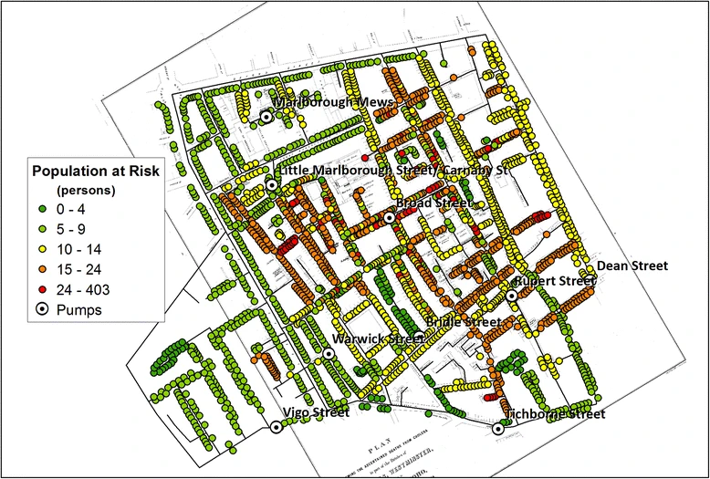
  • John Snow (1855) - cholera epidemic in London tied to a water pump
  • Ronald Ross (1902) - Nobel Prize in Medicine for work on malaria
  • Kermack and McKendrick (1927-1933) - basic epidemic (mathematical) model

Source: Shiode, et al., “The mortality rates and the space-time patterns of John Snow’s cholera epidemic map,” (2015)

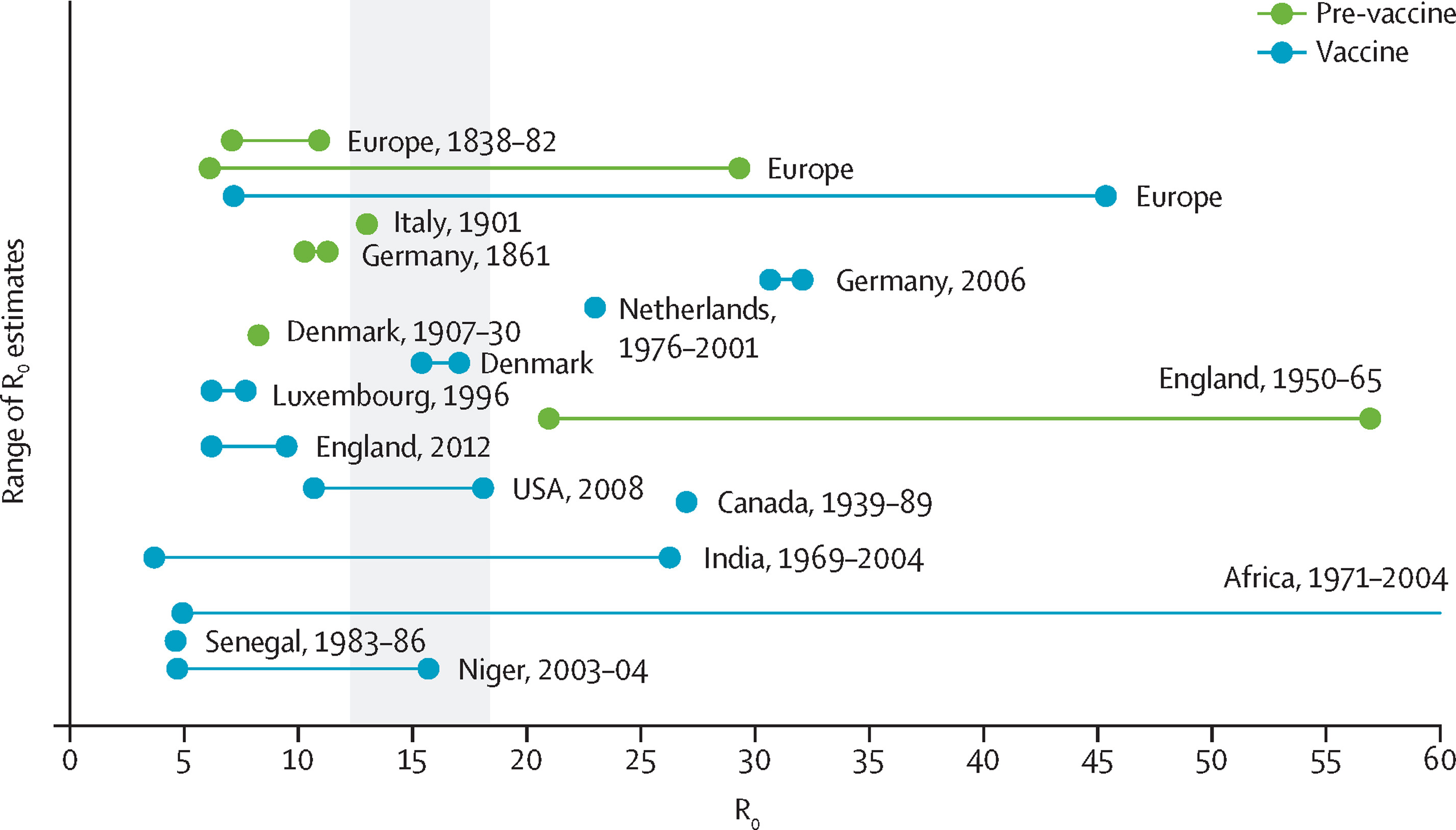
\(R_0\) basic reproduction number

Dates at least to Alfred Lotka (1920s) and others (Feller, Blackwell, etc.)


The expected number of secondary infections due to a primary infection


  • \(R_0 < 1\) the epidemic will die out


  • \(R_0 > 1\) the epidemic will grow until everyone is infected

Source: JHU Measles Tracking Team Data

\(R_0\) is entirely retrospective

  • It’s a property of the pathogen in a fully susceptible (infinite) population

  • Each outbreak is like a new sample


To estimate something like this from data, the “bonehead” way is to

  1. Wait until the epidemic is over (no more infections circulating)
  2. Contact trace the primary infection responsible for each secondary infection
  3. Take a sample average of the number caused by each primary
  4. Possibly repeat over many outbreaks

Source: Guerra, et al., “The basic reproduction number (R0) of measles,” (2019).

Of course no one actually does that


Lots of work on how to estimate \(R_0\)

Effective reproduction number

Suppose \(s\)% of the population is susceptible

Then, “the” effective reproduction number \(R=sR_0\)

Allows you to reason about things like


The level of vaccine coverage necessary to prevent an outbreak from growing uncontrollably.


So, for measles, if \(R_0\approx 15\), the disease will die out if immunity is

\[ sR_0\ \leq\ 1\ \Longrightarrow\ 1-s\ \leq\ 1-\frac{1}{R_0}\ \approx\ 93\% \]

\(R(t)\) — instantaneous reproduction number

  • The effective reproduction number in the middle of an outbreak
  • Some of the population is immune, others are infected, others susceptible

The expected number of secondary infections at time \(t\) caused by an earlier primary infection

  • \(f(a) \geq 0,\ \forall a \geq 0\) — the rate at which an infection of age \(a\) produces new infections

  • \(\displaystyle g(a) := \frac{f(a)} {\int_{0}^\infty f(a)\ \mathsf{d}a} = \frac{f(a)}{R_0}.\)

  • \(\displaystyle R_0 := \int_{0}^\infty f(a)\ \mathsf{d}a.\)

Can allow \(g(t, a)\), hold this fixed for now.

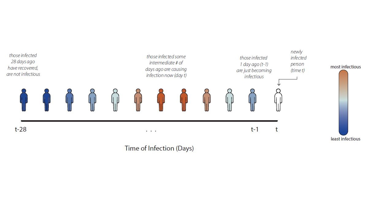
The generation interval distribution \(g(a)\)

Source: US CDC Center for Forecasting Analytics, “Behind the Model.”

SIR-type (compartmental) models - Stochastic Version

Suppose each of N people in a bucket at time t:

Susceptible(t) : not sick, but could get sick

Infected(t) : sick, can make others sick

Removed(t) : recovered or dead; not sick, can’t get sick


  • During period \(h\), each \(S\) meets \(kh\) people.
  • Assume \(\mathbb{P}( S \textrm{ meets } I \textrm{ and becomes } I ) = c\).
  • Then \(\mathbb{P}( S(t) \rightarrow I(t+h) ) = 1 - (1 - c I(t) / N )^{hk} \approx kchI(t) / N\).
  • Therefore, \(I(t+h) \mid S(t),\ I(t) \sim \textrm{Binom}(S(t),\ kchI(t) / N)\).
  • Assume \(\mathbb{P}( I(t) \rightarrow R(t+h)) = \gamma h,\ \forall t\).
  • Then \(R(t+h) \mid I(t) \sim \textrm{Binom}(I(t),\ \gamma h)\).


SIR-type (compartmental) models - Stochastic Version

\[\begin{aligned} x(t+h) &\sim \mathrm{Binom}\left(S(t),\ \frac{\beta}{N} h I(t)\right) = \text{incident infections}\\ z(t+h) &\sim \mathrm{Binom}\left(I(t),\ \gamma h\right) = \text{incident recoveries}\\ S(t+h) & = S(t) - x(t+h)\\ I(t+h) & = I(t) + x(t+h) - z(t+h)\\ R(t+h) & = R(t) + z(t+h) \end{aligned}\]


In the deterministic limit, \(h\rightarrow 0\)

\[\begin{aligned} \frac{\mathsf{d}}{\mathsf{d}t}S(t) & = -\frac{\beta}{N} S(t)I(t)\\ \frac{\mathsf{d}}{\mathsf{d}t}I(t) & = \frac{\beta}{N} I(t)S(t) - \gamma I(t)\\ \frac{\mathsf{d}}{\mathsf{d}t}R(t) & = \gamma I(t) \end{aligned}\]


THE SIR model is often ambiguous between these.

Typically, people mean the deterministic, continuous time version.

\(R_t\) in compartmental models

There is an equivalence between a compartmental model and the renewal equation.

\[\begin{aligned} R_0 &= \beta\ /\ \gamma\\ x_{t+1} &= \beta \frac{S_{t}}{N} \sum_{k = 0}^{t-1} \big[(1-\gamma)^{k}\big] x_{t-k} = R_0 \frac{S_{t}}{N} \sum_{k = 0}^{t-1} \big[\gamma(1-\gamma)^{k}\big] x_{t-k} = R_{t}\sum_{k = 0}^{t-1} g(k)x_{t-k} \end{aligned}\]

\(R(t)\) and \(R_t\) — renewal equation

Alternatively: rather than working with a particular compartmental model

Define \(R(t)\) implicitly through the renewal equation

\[ x(t) = R(t)\int_0^\infty x(t-a)g(a)\mathsf{d}a = R(t)\times (x * g)(t), \]

where \(x(t)\) are infections at time \(t\).


In discrete time,

\[ x_{t+1} = R_t\sum_{a=0}^\infty x_{t-a}\widetilde{g}_a = R_t\times (x * \widetilde{g})_t. \]


And stochasticly,

\[ \mathbb{E}\big[x_{t+1} \mid x_1,\ldots,x_{t}\big] = R_t\sum_{a=0}^\infty x_{t-a}\widetilde{g}_a = R_t\times (x * \widetilde{g})_t. \]

Most estimators start here: \[ \mathbb{E}\big[x_{t+1} \mid x_1,\ldots,x_{t}\big] = R_t\sum_{a=0}^\infty x_{t-a}\widetilde{g}_a. \]

  • Assume \(\widetilde{g}\) is known
  • Model \(x_{t+1} \mid x_1,\ldots,x_{t}\) as Poisson or Negative Binomial
  • Turn some inferential crank

\(R_t\) for Influenza

Source: US CDC Center for Forecasting Analytics

Estimating \(R_t\)

Data issues

\(x_t\) is incident infections, but we don’t ever see those

Source: US CDC Center for Forecasting Analytics, “Behind the Model.”
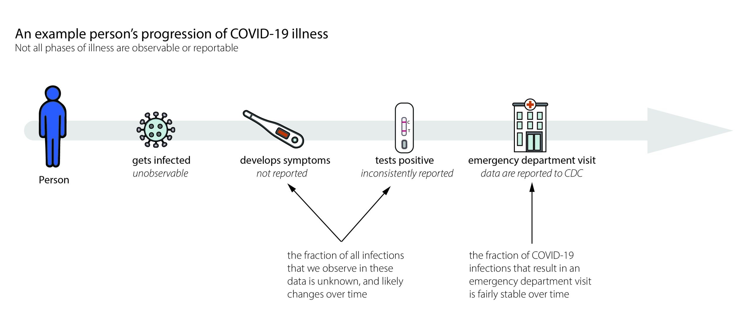
  • Replace infections with cases
  • Replace generation interval with serial interval
  • Assume we have the serial interval

Serial interval distribution


Standard model for \(R_t\)

\[\begin{aligned} \eta_t &= \sum_{a=0}^{t-1} y_{t-a}p_a,\\ \\ y_t\ |\ y_{t-1},\ldots,y_{1} &\sim \textrm{Poisson}(R_t\eta_t). \end{aligned}\]

  • Using \(y\) instead of \(x\) to be cases or hospitalizations or deaths, incidence
  • Using \(p\) for serial interval distribution (discretized)
  • The MLE for \(R_t\) is just \(y_t / \eta_t\).
  • This has really high variance, but unbiased.
  • So everybody smooths it.
  • This isn’t going to give you “\(R_t\)”, because you didn’t use incident infections.

  • At least, the timing is wrong, because the observable happened after infection.

  • Better to deconvolve incidence first (LSM2026).

More on this later.

The state of the art

  1. {EpiEstim} CFFC2013
  • Gamma prior on \(R_t\), but use a trailing window
  • Super fast computationally
  • Smoothness is ad hoc
  1. {EpiFilter} Parag 2020
  • State space model
  • One step smoothness: \(R_{s+1} \sim \textrm{Gaussian}(R_s,\ \alpha R_s)\)
  • Uses a discretized particle filter-type algorithm
  1. {EpiLPS} GFH2023
  • Negative Binomial likelihood
  • Smoothness via \(\log(R_t\eta_t) = \mathbf{B}_{t,:}\beta\)
  • \(\mathbf{B}\) is cubic B-spline basis, weighted Ridge penalty on \(\beta\)
  • More priors, use Metropolis Adjusted Langevin Algorithm

{EpiNow2} CDC + CFA, Abbott, et al., 2023

  • Negative Binomial likelihood
  • Smoothness via a GP prior
  • Accommodates the sequence of delays from infection \(\longrightarrow\) ??
  • Adjusts for real-time issues like partial reporting
  • Big Bayesian MCMC in Stan. Very slow.

Our model

Let \(\theta_t := \log(R_t)\).

Use Poisson likelihood.

\[ \begin{aligned} \widehat{R} &= \exp(\widehat{\theta}) &\widehat{\theta} &= \mathop{\mathrm{argmin}}_\theta\; \eta^{\mathsf{T}}\exp(\theta) - \mathbf{y}^{\mathsf{T}}\theta + \lambda\Vert D^{(k+1)}\theta\Vert_1 \end{aligned} \]

  • Convex, has a global optimum
  • \(\lambda\) controls smoothness relative to data fidelity
  • \(\ell_1\) penalty produces adaptive piecewise polynomials of order \(k+1\)
  • Near minimax optimal for functions with bounded total variation

Local adaptivity — \(\ell_1\) vs. \(\ell_2\)

Polynomial order, \(k=0\)


\[ \begin{aligned} D^{(1)} &= \begin{bmatrix} 1 & -1 & & & & \\ & 1 & -1 & & & \\ & & & \ddots && \\ & & & & 1 & -1 \end{bmatrix} \\ \\ &\in \mathbb{R}^{(n-1)\times n} \end{aligned} \]

Polynomial order, \(k=1\)


\[ \begin{aligned} D^{(2)} &= \begin{bmatrix} 1 & -2 & 1 & & & \\ & 1 & -2 & 1 & & \\ & & & \ddots && \\ & & & 1 & -2 & 1 \end{bmatrix} \\ \\ &= D^{(1)}D^{(1)}\\ \\ &\in \mathbb{R}^{(n-k-1)\times n} \end{aligned} \]

Polynomial order, \(k=2\)


\[\begin{aligned} D^{(3)} &= \begin{bmatrix} -1 & 3 & -3 & 1 & & \\ & -1 & 3 & -3 &1 & \\ & & & \ddots && \\ & & -1 & 3 & -3 & 1 \end{bmatrix} \\ \\ &= D^{(1)}D^{(2)}\\ \\ &\in \mathbb{R}^{(n-k-1)\times n} \end{aligned}\]

Estimation algorithm

\[\mathop{\mathrm{minimize}}_\theta\; \eta^{\mathsf{T}}\exp(\theta) - \mathbf{y}^{\mathsf{T}}\theta + \lambda\Vert D^{(k+1)}\theta\Vert_1\]

Estimation algorithm

\[\mathop{\mathrm{minimize}}_{\theta,\ {\color{BurntOrange} \alpha}}\; \eta^{\mathsf{T}}\exp(\theta) - \mathbf{y}^{\mathsf{T}}\theta + \lambda\Vert D^{(1)}{\color{BurntOrange} \alpha}\Vert_1\quad {\color{BurntOrange} \textrm{subject to}\quad \alpha = D^{(k)}\theta}\]

Estimation algorithm

\[\mathop{\mathrm{minimize}}_{\theta,\ \alpha}\; \eta^{\mathsf{T}}\exp(\theta) - \mathbf{y}^{\mathsf{T}}\theta + \lambda\Vert D^{(1)} \alpha\Vert_1\quad \textrm{subject to}\quad \alpha = D^{(k)}\theta\]


Alternating direction method of multipliers (ADMM)

\[\begin{aligned} \theta &\longleftarrow \mathop{\mathrm{argmin}}_\theta\ \eta^{\mathsf{T}}\exp(\theta) - \mathbf{y}^{\mathsf{T}}\theta + \frac{\rho}{2}\Vert D^{(k)}\theta - \alpha + u \Vert_2^2 \\ \alpha &\longleftarrow \mathop{\mathrm{argmin}}_\alpha\ \lambda\Vert D^{(1)} \alpha \Vert_1 + \frac{\rho}{2}\Vert D^{(k)}\theta - \alpha + u \Vert_2^2 \\ u &\longleftarrow u + D^{(k)}\theta - \alpha \end{aligned}\]

Estimation algorithm

\[\mathop{\mathrm{minimize}}_{\theta,\ \alpha}\; \eta^{\mathsf{T}}\exp(\theta) - \mathbf{y}^{\mathsf{T}}\theta + \lambda\Vert D^{(1)} \alpha\Vert_1\quad \textrm{subject to}\quad \alpha = D^{(k)}\theta\]


Alternating direction method of multipliers (ADMM)

\[\begin{aligned} \theta &\longleftarrow \Big[{\color{Cerulean}\textrm{Proximal Newton / Fisher Scoring}}\Big] \\ \alpha &\longleftarrow \Big[{\color{BurntOrange}\textrm{Fused Lasso Signal Approximator}}\Big] \\ u &\longleftarrow u + D^{(k)}\theta - \alpha \end{aligned}\]

Solve sequentially for \(\Vert (D^{\dagger})^{\mathsf{T}}(\eta - y)\Vert_\infty = \lambda_1 > \cdots > \lambda_M=\epsilon \lambda_1\).

Results and features

Canadian Covid-19 cases

\(R_t\) for Canadian Covid-19 cases

Reconvolved Canadian Covid-19 cases

Example simulations for different methods

{rtestim} software

  • Guts are in C++ for speed

  • Lots of the usual S3 methods

  • Approximate “confidence” bands

  • \(\widehat{R}\) is a member of a function space

  • Arbitrary spacing of observations

  • Built-in cross validation

  • Time-varying delay distributions

{rtestim} software

  • Guts are in C++ for speed

  • Lots of the usual S3 methods

  • Approximate “confidence” bands

  • \(\widehat{R}\) is a member of a function space

  • Arbitrary spacing of observations

  • Built-in cross validation

  • Time-varying delay distributions

Approximation + Delta method gives

\[ \textrm{Var}(\widehat{R}) = \left(\textrm{diag}(\widehat{y}) + \lambda D^{\mathsf{T}}D\right)^{\dagger} \left(\frac{1}{\eta^2}\right) \]

{rtestim} software

  • Guts are in C++ for speed

  • Lots of the usual S3 methods

  • Approximate “confidence” bands

  • \(\widehat{R}\) is a member of a function space

  • Arbitrary spacing of observations

  • Built-in cross validation

  • Time-varying delay distributions

The solution is an element of the space of discrete splines of order \(k\) Tibshirani 2020

  • Lets us interpolate (and extrapolate) to off-observation points
  • Lets us handle uneven spacing

{rtestim} software

  • Guts are in C++ for speed

  • Lots of the usual S3 methods

  • Approximate “confidence” bands

  • \(\widehat{R}\) is a member of a function space

  • Arbitrary spacing of observations

  • Built-in cross validation

  • Time-varying delay distributions

{rtestim} software

Summary and collaborators

Contributions

  • Framework for \(R_t\) estimation
  • Naturally imposes smoothness
  • Fast, extensible, easy to use
  • Has “confidence” bands

Future work

  • Allow Negative Binomial likelihood
  • Deconvolve incidence
  • Forecast
  • Mixed smoothness behaviours
  • Figure out CV for convolution
  • Better confidence bands
  • Use relationship with growth rate

Collaborators and funding