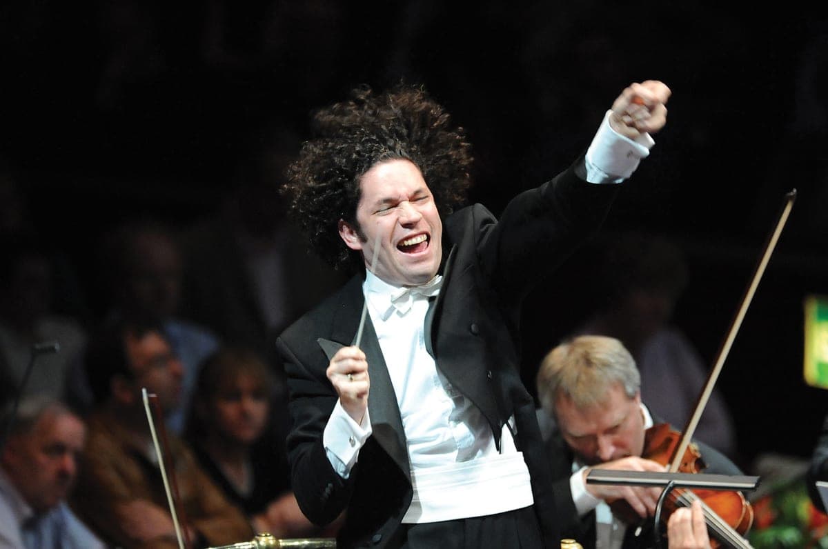
Markov-Switching Models for Musical Interpretation

Daniel J. McDonald

• Dabbled in Economics
• PhD is Statistics
• IU happened to have an opening
• Met Prof. Chris Raphael at my interview
• Accepted the Job
• Occasionally dabbled in Music on the Side
• First invited talk at Laval on Music
• Finally published the paper in 2021

Musical taste

• Easy to describe music you like:

  • “Jazzy sound”

  • “Strong beat”

  • “good lyrics”

  • “anything by Taylor Swift”

• Harder to describe a performance

• Classical music is mainly about performances of the same music

How do we think about which ones we like?

Primer on “classical” music

• Written between 6th century and today
• Includes music written during the Classical period (1750–1820)

The real difference is that when a composer writes a piece of what’s usually called classical music, he puts down the exact notes that he wants, the exact instruments or voices that he wants to play or sing those notes—even the exact number of instruments or voices; and he also writes down as many directions as he can think of.

–Leonard Bernstein

Generally much more musically complicated

• Musically complicated = wider range of chords, keys, instrumentation, contrasts
• Hey Jude: 3 chords (2 others briefly) in 7 minutes. Same key the whole time.
• For today, Chopin is running example
• Chopin: 6 unique chords in first 10 seconds. Two key areas in 1.5 minutes of music.

What’s different?

1. Mistakes
2. Extraneous noise
3. Recording quality
4. Articulation / Legato / Bowing / Breathing
5. Dynamics
6. Tempo / Rubato

Source: WBUR Boston

The first three are uninteresting.

The others are about interpretation

We like performances with “better” interpretations

Piano music

• Simplifies the problem
  • No bowing, fingering, breathing, glissando
• Focus on tempo
• professional pianists would cringe as I say this, but contrast with strings / winds / singers
• This is Drake’s Piano

Musical tempo

• Notes change speed

• Sometimes purposeful

• Speed is important for interpretation

• Orange is Rubinstein, as recorded
• Dashed is “mine”, mechanically forced Rubinstein to be constant speed
• Mention axes
• Note the “slow down” at the end (phrase boundary)

What is this “music”?

Important musical terms

Notes

Beat

Measure

Time signature

Tempo

Dynamics

All those little black dots

Strongly felt impetus

Collections of notes delimited by vertical “barlines”

Number of beats / measure; type of note that gets the beat

The prevailing speed, measured in bpm

Loudness of the note

• notes indicate pitch and relative duration
• (relative to…) beat is the baseline
• accents / pedal markings

Data

• CHARM Mazurka Project

• Focus on timing only (dynamics also available)

• 50 recordings: Chopin Mazurka Op. 68 No. 3

• Recorded between 1931 and 2006

• 45 different performers

• Note the shaded region

Chopin & Mazurkas

Fryderyk Chopin (1810–1849)

• Born in Poland

• Moved to Paris at 21

• Virtuoso pianist

• Wrote mainly piano music

Mazurka

• A Polish dance

• Chopin composed at least 58 for Piano

• Repetition is very important

• Certain rhythmic figures

Everything he wrote includes piano

• Recording by Christoph Zbinden, available from the IMSLP under CC By 4.0.
• Tempo markings, importantly, only 2 + rit and fermata
• Dotted eighth sixteenth
• ABA structure
• Minor phrases
• Repetition
• Chord progression

Modelling tempo

Tempo regimes

1. Constant tempo

2. Accelerando (speeding up)

3. Ritarando (slowing down)

4. Tenuto (emphasis)

Transition diagram

1. Constant tempo

2. Accelerando (speeding up)

3. Ritarando (slowing down)

4. Tenuto (emphasis)

• Can jump “right back”
• What’s the difference between 1-3-1, 1-4-1?

Transition diagram

1. Constant tempo

2. Accelerando (speeding up)

3. Ritarando (slowing down)

4. Tenuto (emphasis)

Before \(|\mathcal{S}| = 4\). Now, \(|\mathcal{S}| = 11\)

• No longer 1-Markov
• Any K-Markov can be made 1-Markov by expanding state-space
• Now \(J=11\) states

The HMM

HMM Inference

Viterbi algorithm gives estimates of \(\{S_k\}\)

Computation is \(O(n)\): likelihood of \(p\) and estimates of \(\{S_k\}\)

Inside of EM (Baum-Welch) gives estimates of \(p\)

• Not enough flexibility
• Return to Constant needs new tempo
• “Noise around intended tempo” vs “Noise in intentions”

Intentions vs. observations

• Musicians aren’t perfect.
• Imagine a speed that they’ll maintain in CT state.
• Accelerate/Decel from there.
• Need to track tempo/accel in \(X_k\).
• These depend on \(S_k\) and \(S_{k-1}\)
• Observe noisy realization

Switching Kalman filter

Kalman filter algorithm

• Developed in the late 1950s to track missiles

\[ \begin{aligned} X_{k+1} &= d_k + T_k X_k + \eta_{k+1}, & \eta_{k+1} &\sim \textrm{N}(0, Q_{k+1}),\\ Y_k &= c_k + Z_k X_k + \epsilon_{k}, &\epsilon_k & \sim \textrm{N}(0, G_k).\\ \end{aligned} \]

• Assume \(X_0\) is Gaussian

• KF just tracks mean and variance of \(X_k\ |\ \{Y_i\}_{i=1}^k\)

• Does this iteratively for each \(k\)

• kfilter() gives estimate of \(\{X_k\; |\; Y_1,\ldots,Y_k\}_{k=1}^n\)

• kfilter() also gives likelihood of \(\theta\)

• ksmoother() gives estimate of \(\{X_k\; |\; Y_1,\ldots,Y_n\}_{k=1}^n\)

Photographer: Anas Baba/AFP/Getty Images

Kalman filter inference

\[ \begin{aligned} X_{k+1} &= {\color{Plum} d_k} + {\color{Plum} T_k} X_k + \eta_{k+1}, & \eta_{k+1} &\sim \textrm{N}(0, {\color{Plum} Q_{k+1}}),\\ Y_k &= {\color{Plum} c_k} + {\color{Plum} Z_k} X_k + \epsilon_{k}, &\epsilon_k & \sim \textrm{N}(0, {\color{Plum} G_k}).\\ \end{aligned} \]

Parameter matrices may depend on

• Parameter vector \(\theta\)
• Current or previous values of \(X\) and \(Y\)

Kalman filter inference

\[ \begin{aligned} X_{k+1} &= {\color{Plum} d_k} + {\color{Plum} T_k} X_k + \eta_{k+1}, & \eta_{k+1} &\sim \textrm{N}(0, {\color{Plum} Q_{k+1}}),\\ Y_k &= {\color{Plum} c_k} + {\color{Plum} Z_k} X_k + \epsilon_{k}, &\epsilon_k & \sim \textrm{N}(0, {\color{Plum} G_k}).\\ \end{aligned} \]

kfilter() \(+\) ksmoother() algorithms gives estimates of \(\{X_k\}\)

Computation is \(O(n)\): likelihood of \(\theta\) and estimates of \(\{X_k\}\)

Inside of EM gives estimates of \(\theta\)

Switching Kalman filter (for our model)

\[ \begin{aligned} X_{k} &= d(s_k,\ s_{k-1}) + T(s_k,\ s_{k-1}) X_{k-1} + \eta_{k}\\\\ Y_k &= c(s_k) + Z(s_k) X_k + \epsilon_{k}\\\\ \eta_{k} &\sim \textrm{N}(0, Q(s_k,\ s_{k-1}))\\\\ \epsilon_k & \sim \textrm{N}(0, G(s_k)) \end{aligned} \]

We want to estimate: \(\theta\), \(p\), \(\{X_k\}\), and \(\{S_k\}\)

This costs \(O(|\mathcal{S}|^n)\), \(|\mathcal{S}|=11\), \(n=231\)

The problem is all the paths through the states

We don’t know the path through the discrete states

• I have 4 states
• 2nd order Markov
• Leads to 11 states in 1-Markov
• Piece has 231 notes

Discrete particle filter — dpf()

Track at most \(J\) paths through the \(|\mathcal{S}|^n\) tree

1. At time \(k\), receive \(J\) paths: a state sequence and a weight

2. Propagate each of the \(J\) paths forward, creating \(\approx J^2\)

3. Using the weights, sample the \(\approx J^2\) possibilities to get only \(J\)

4. iterate forward through time until done, return \(J\) sequences and their weights

• This is a greedy approximation
• AKA “Beam Search”
• The sampling step is important
• Probability of sampling is proportional to current weight \(\times\) likelihood \(\times\) trans prob
• Example supposing \(J = 5\)

The complete pseudocode

For each performance:

• Iterate 1–3 to maximize for \(\theta \in \Theta\), produce \(\widehat\theta\)
  1. Guess a parameter vector \(\theta\) (in some sensible way)
  2. dpf() gives greedy state sequence \(\{\widehat{S}_k\}_{k=1}^n\)
  3. It gives the likelihood as a side effect via kfilter()
• Rerun dpf() and ksmoother() at \(\widehat{\theta}\) to get \(\{\widehat{S}_k\}_{k=1}^n\) and \(\{\widehat{X}_k\}_{k=1}^n\)

• Takes a few minutes per performance when 1 is done intelligently
• I used 6hr walltime on Cedar with 1 perf / core and 10 restarts

Decoding mazurkas

The estimated parameters

For each performance, we estimate \(p\) and \(\theta\) by penalized maximum likelihood.

Abuse notation and redefine \(\theta := (p, \theta)\)

• average speed in different states

• some variance parameters

• transition probabilities

We have strong prior information.

Examples of strong priors

Distance matrix on parameters

Use Mahalanobis \[d(\theta,\theta') = \sqrt{(\theta-\theta')^\mathsf{T} \mathbf{V}^{-1}(\theta-\theta')}\]

\(\mathbf{V}\) is prior covariance matrix

Incorporates correlations correctly on probability vectors

Some performances have no close neighbors

Probability of “stress”

Cluster 1

Cluster 2

Similar performances

Arthur Rubinstein

Cortot?

• Not actually Cortot
• Likely Hatto or perhaps even an engineered recording
• This was a major scandal for the British Concert Artist record label in about 2006/7
• about 100 other fake recordings
• Discovered by uploading to Gracenote database

In summary

• We develop a switching model for tempo decisions

• We give an algorithm for performing likelihood inference

• We estimate our model using a large collection of recordings of the same composition

• We demonstrate how the model is able to recover performer intentions

• We use the learned representations to compare and contrast recordings

Future work

• Similar model for dynamics

• Can we do this fast and “online”?

• Use it for teaching?

Collaborators, funding, etc.

Christopher Raphael

Michael McBride

 

Rob Granger