{epiprocess} and {epipredict}

R packages for signal processing and forecasting


Daniel J. McDonald, Ryan J. Tibshirani, and Logan C. Brooks

and CMU’s Delphi Group

CDC Flu Site Visit — 19 July 2023

Background

  • Covid-19 Pandemic required quickly implementing forecasting systems.
  • Basic processing—outlier detection, reporting issues, geographic granularity—implemented in parallel / error prone
  • Data revisions complicate evaluation
  • Simple models often outperformed complicated ones
  • Custom software not easily adapted / improved by other groups
  • Hard for public health actors to borrow / customize community techniques

Packages under development

flowchart LR
  A("{epidatr}") --> C("{epiprocess}")
  B("{epidatpy}") --> C
  D("{covidcast}") --> C
  C --> E("{epipredict}")

{epiprocess}

Tools for signal processing

Basic processing operations and data structures

  • General EDA for panel data
  • Calculate rolling statistics
  • Fill / impute gaps
  • Examine correlations, growth rates
  • Store revision history smartly
  • Inspect revision patterns
  • Find / correct outliers

epi_df: snapshot of a data set

  • a tibble; requires columns geo_value and time_value.
  • arbitrary additional columns containing measured values
  • additional keys to index (age_group, ethnicity, etc.)

epi_df

Represents a snapshot that contains the most up-to-date values of the signal variables, as of a given time.

epi_df: snapshot of a data set

Example data object documentation, license, attribution
case_death_rate_subset       package:epipredict        R Documentation

Subset of JHU daily state cases and deaths

Description:

     This data source of confirmed COVID-19 cases and deaths is based
     on reports made available by the Center for Systems Science and
     Engineering at Johns Hopkins University. This example data ranges
     from Dec 31, 2020 to Dec 31, 2021, and includes all states.

Usage:

     case_death_rate_subset
     
Format:

     A tibble with 20,496 rows and 4 variables:

     geo_value the geographic value associated with each row of
          measurements.

     time_value the time value associated with each row of
          measurements.

     case_rate 7-day average signal of number of new confirmed COVID-19
          cases per 100,000 population, daily

     death_rate 7-day average signal of number of new confirmed deaths
          due to COVID-19 per 100,000 population, daily

Source:

     This object contains a modified part of the COVID-19 Data
     Repository by the Center for Systems Science and Engineering
     (CSSE) at Johns Hopkins University as republished in the COVIDcast
     Epidata API. This data set is licensed under the terms of the
     Creative Commons Attribution 4.0 International license by the
     Johns Hopkins University on behalf of its Center for Systems
     Science in Engineering. Copyright Johns Hopkins University 2020.

     Modifications:

        • From the COVIDcast Epidata API: These signals are taken
          directly from the JHU CSSE COVID-19 GitHub repository without
          changes. The 7-day average signals are computed by Delphi by
          calculating moving averages of the preceding 7 days, so the
          signal for June 7 is the average of the underlying data for
          June 1 through 7, inclusive.

An `epi_df` object, 20,496 x 4 with metadata:
* geo_type  = state
* time_type = day
* as_of     = 2022-05-31 12:08:25.791826

# A tibble: 20,496 × 4
   geo_value time_value case_rate death_rate
 * <chr>     <date>         <dbl>      <dbl>
 1 ak        2020-12-31      35.9      0.158
 2 al        2020-12-31      65.1      0.438
 3 ar        2020-12-31      66.0      1.27 
 4 as        2020-12-31       0        0    
 5 az        2020-12-31      76.8      1.10 
 6 ca        2020-12-31      96.0      0.751
 7 co        2020-12-31      35.8      0.649
 8 ct        2020-12-31      52.1      0.819
 9 dc        2020-12-31      31.0      0.601
10 de        2020-12-31      65.2      0.807
# ℹ 20,486 more rows

Sliding examples on epi_df

Correlations at different lags

cor0 <- epi_cor(edf, case_rate, death_rate, cor_by = time_value)
cor14 <- epi_cor(edf, case_rate, death_rate, cor_by = time_value, dt1 = -14)

Outlier detection and correction

ny <- ny %>% mutate(outliers = detect_outlr_stl(time_value, cases))

Sliding examples on epi_df

Growth rates

edf <- filter(edf, geo_value %in% c("ut", "ca")) %>%
  group_by(geo_value) %>%
  mutate(gr_cases = growth_rate(time_value, case_rate, method = "trend_filter"))

epi_archive: collection of epi_dfs

  • full version history of a data set
  • acts like a bunch of epi_dfs — but stored compactly
  • allows similar funtionality as epi_df but using only data that would have been available at the time

Revisions

Epidemiology data gets revised frequently. (Happens in Economics as well.)

  • We may want to use the data as it looked in the past
  • or we may want to examine the history of revisions.

Revision patterns

Example data object documentation, license, attribution
archive_cases_dv_subset       package:epiprocess       R Documentation

Subset of daily doctor visits and cases in archive format

Description:

     This data source is based on information about outpatient visits,
     provided to us by health system partners, and also contains
     confirmed COVID-19 cases based on reports made available by the
     Center for Systems Science and Engineering at Johns Hopkins
     University. This example data ranges from June 1, 2020 to Dec 1,
     2021, and is also limited to California, Florida, Texas, and New
     York.

Usage:

     archive_cases_dv_subset
     
Format:

     An 'epi_archive' data format. The data table DT has 129,638 rows
     and 5 columns:

     geo_value the geographic value associated with each row of
          measurements.

     time_value the time value associated with each row of
          measurements.

     version the time value specifying the version for each row of
          measurements.

     percent_cli percentage of doctor’s visits with CLI (COVID-like
          illness) computed from medical insurance claims

     case_rate_7d_av 7-day average signal of number of new confirmed
          deaths due to COVID-19 per 100,000 population, daily

Source:

     This object contains a modified part of the COVID-19 Data
     Repository by the Center for Systems Science and Engineering
     (CSSE) at Johns Hopkins University as republished in the COVIDcast
     Epidata API. This data set is licensed under the terms of the
     Creative Commons Attribution 4.0 International license by Johns
     Hopkins University on behalf of its Center for Systems Science in
     Engineering. Copyright Johns Hopkins University 2020.

     Modifications:

        • From the COVIDcast Doctor Visits API: The signal
          'percent_cli' is taken directly from the API without changes.

        • From the COVIDcast Epidata API: 'case_rate_7d_av' signal was
          computed by Delphi from the original JHU-CSSE data by
          calculating moving averages of the preceding 7 days, so the
          signal for June 7 is the average of the underlying data for
          June 1 through 7, inclusive.

        • Furthermore, the data is a subset of the full dataset, the
          signal names slightly altered, and formatted into a tibble.

Latency investigation

How stale is my data over space and time?

There are (lots) of possible definitions.

Nominal latency
the difference between the max time_value available for some location, as of some version
Nonmissing latency
nominal + recorded NAs and skipped time_values are latent
Nonmissing nonzero latency
nonmissing + zeros are latent
Nonmissing nonduplicate latency
nonmissing + duplications of the most recent non-NA values are latent

Latency investigation

pos_first_true <- function(x) match(TRUE, rev(x), length(x) + 1) - 1

na0_latency <- function(dat, group_key, ref_time_value) {
  group_by(dat, geo_value) %>%
    complete(time_value = full_seq(time_value, period = 1L)) %>%
    mutate(not_na0 = !(is.na(admissions) | admissions == 0L)) %>%
    summarize(
      nominal_latency = as.integer(ref_time_value - max(time_value)),
      na0_latency = pos_first_true(not_na0) + nominal_latency
    )
}

hhs_flu_hosp_archive %>% 
  epix_slide(na0_latency, before = 27, names_sep = NULL) %>% 
  rename(version = time_value)

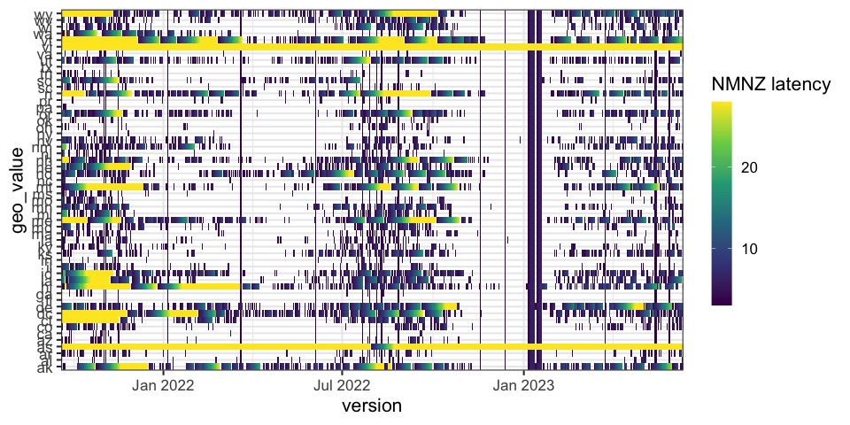
Latency investigation, > 2 days

{epipredict}

A forecasting framework

Philosophy of forecasting

We should build up modular components

Be able to add layers sequentially

  1. Preprocessor: do things to the data before model training
  2. Trainer: train a model on data, resulting in an object
  3. Predictor: make predictions, using a fitted model object
  4. Postprocessor: do things to the predictions before returning

A very specialized plug-in to {tidymodels}

{epipredict}

  • Canned forecasters that work out-of-the-box
  • Backtest using the versioned data
  • Easily create features
  • Modify / transform / calibrate forecasts
  • Quickly pivot to new tasks
  • Highly customizable for advanced users

Canned forecasters that work out of the box.

But, you can adjust a lot of options

We currently provide:

  • Baseline flat-line forecaster
  • Autoregressive-type forecaster
  • Autoregressive-type classifier
  • “Smooth” autoregressive-type forecaster

Canned forecasters that work out of the box.

But, you can adjust a lot of options

Example forecasting task

  • On day \(t\)

  • We want to predict

    • new hospitalizations \(y\),
    • \(h\) days ahead,
    • at many locations \(j\).
  • We’re going to make a new forecast each week.

Canned forecasters that work out of the box.

But, you can adjust a lot of options

Flatline forecaster

For each location, predict \[\hat{y}_{j,\ t+h} = y_{j,\ t}\]

Canned forecasters that work out of the box.

But, you can adjust a lot of options

AR forecaster

Use an AR model with an extra feature, e.g.: \[\hat{y}_{j,\ t+h} = \mu + a_0 y_{j,\ t} + a_7 y_{j,\ t-7} + b_0 x_{j,\ t} + b_7 x_{j,\ t-7}\]

Basic autoregressive forecaster

  • Predict death_rate, 1 week ahead, with 0,7,14 day lags of cases and deaths.
  • Use lm for estimation. Also create intervals.
edf <- case_death_rate_subset # grab some built-in data
canned <- arx_forecaster(
  epi_data = edf, 
  outcome = "death_rate", 
  predictors = c("case_rate", "death_rate")
)

The output is a model object that could be reused in the future, along with the predictions for 7 days from now.

Adjust lots of built-in options

rf <- arx_forecaster(
  epi_data = edf, 
  outcome = "death_rate", 
  predictors = c("case_rate", "death_rate", "fb-survey"),
  trainer = parsnip::rand_forest(mode = "regression"), # use {ranger}
  args_list = arx_args_list(
    ahead = 14, # 2-week horizon
    lags = list(
      case_rate = c(0:4, 7, 14), 
      death_rate = c(0, 7, 14), 
      `fb-survey` = c(0:7, 14)
    ),
    levels = c(0.01, 0.025, 1:19/20, 0.975, 0.99), # 23 ForecastHub quantiles
    quantile_by_key = "geo_value" # vary noise model by location
  )
)

Do (almost) anything manually

# A preprocessing "recipe" that turns raw data into features / response
r <- epi_recipe(edf) %>%
  step_epi_lag(case_rate, lag = c(0, 1, 2, 3, 7, 14)) %>%
  step_epi_lag(death_rate, lag = c(0, 7, 14)) %>%
  step_epi_ahead(death_rate, ahead = 14) %>%
  step_epi_naomit()

# A postprocessing routine describing what to do to the predictions
f <- frosting() %>%
  layer_predict() %>%
  layer_threshold(.pred, lower = 0) %>% # predictions / intervals should be non-negative
  layer_add_target_date(target_date = max(edf$time_value) + 14) %>%
  layer_add_forecast_date(forecast_date = max(edf$time_value))

# Bundle up the preprocessor, training engine, and postprocessor
# We use quantile regression
ewf <- epi_workflow(r, quantile_reg(tau = c(.1, .5, .9)), f)

# Fit it to data (we could fit this to ANY data that has the same format)
trained_ewf <- ewf %>% fit(edf)

# examines the recipe to determine what we need to make the prediction
latest <- get_test_data(r, edf)

# we could make predictions using the same model on ANY test data
preds <- trained_ewf %>% predict(new_data = latest)

Visualize a result for 1 forecast date, 1 location

Code
fd <- as.Date("2021-11-30")
geos <- c("ut", "ca")

tedf <- edf %>% filter(time_value >= fd)
# use most recent 3 months for training
edf <- edf %>% filter(time_value < fd, time_value >= fd - 90L)

rec <- epi_recipe(edf) %>%
  step_epi_lag(case_rate, lag = c(0, 7, 14, 21)) %>%
  step_epi_lag(death_rate, lag = c(0, 7, 14)) %>%
  step_epi_ahead(death_rate, ahead = 1:28)

f <- frosting() %>%
  layer_predict() %>%
  layer_unnest(.pred) %>%
  layer_naomit(distn) %>%
  layer_add_forecast_date() %>%
  layer_threshold(distn)

ee <- smooth_quantile_reg(
  tau = c(.1, .25, .5, .75, .9),
  outcome_locations = 1:28,
  degree = 3L
)

ewf <- epi_workflow(rec, ee, f)
  
the_fit <- ewf %>% fit(edf)

latest <- get_test_data(rec, edf, fill_locf = TRUE)
preds <- predict(the_fit, new_data = latest) %>%
  mutate(forecast_date = fd, target_date = fd + ahead) %>%
  select(geo_value, target_date, distn) %>%
  pivot_quantiles(distn) %>%
  filter(geo_value %in% geos)

ggplot(preds) +
  geom_ribbon(aes(target_date, ymin = `0.1`, ymax = `0.9`),
              fill = "cornflowerblue", alpha = .8) +
  geom_ribbon(aes(target_date, ymin = `0.25`, ymax = `0.75`),
              fill = "#00488E", alpha = .8) +
  geom_line(data = bind_rows(tedf, edf) %>% filter(geo_value %in% geos), 
            aes(time_value, death_rate), size = 1.5) +
  geom_line(aes(target_date, `0.5`), color = "orange", size = 1.5) +
  geom_vline(xintercept = fd) +
  facet_wrap(~geo_value) +
  theme_bw(16) +
  scale_x_date(name = "", date_labels = "%b %Y") +
  ylab("Deaths per 100K inhabitants")

Questions?