sim_SIR <- function(TT, N = 1000, beta = .1, gamma = .01) {

  S <- double(TT)
  I <- double(TT)
  R <- double(TT)
  S[1] <- N - 1
  I[1] <- 1

  for (tt in 2:TT) {
    contagions <- rbinom(1, size = S[tt - 1], prob = beta * I[tt - 1] / N)
    removals <- rbinom(1, size = I[tt - 1], prob = gamma)
    S[tt] <- S[tt - 1] - contagions
    I[tt] <- I[tt - 1] + contagions - removals
    R[tt] <- R[tt - 1] + removals
  }
  tibble(S = S, I = I, R = R, time = seq(TT))
}CANSSI Prairies — Epi Forecasting Workshop 2025
Compartmental Models, Renewal Equations, and \(R_t\) Estimation
Lecture 3
Mathematical modelling of disease / epidemics is very old
Daniel Bernoulli (1760) - studies inoculation against smallpox
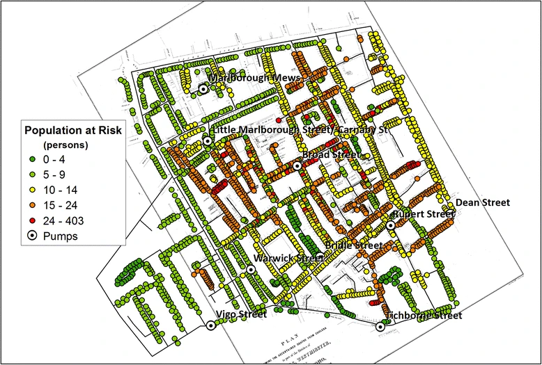
John Snow (1855) - cholera epidemic in London tied to a water pump
Ronald Ross (1902) - Nobel Prize in Medicine for work on malaria
Kermack and McKendrick (1927-1933) - basic epidemic (mathematical) model
SIR-type (compartmental) models - Stochastic Version
Suppose each of N people in a bucket at time t:
Susceptible(t) : not sick, but could get sick
Infected(t) : sick, can make others sick
Removed(t) : recovered or dead; not sick, can’t get sick
- During period \(h\), each \(S\) meets \(kh\) people.
- Assume \(P( S \textrm{ meets } I \textrm{ and becomes } I ) = c\).
- Then \(P( S(t) \rightarrow I(t+h) ) = 1 - (1 - c I(t) / N )^{hk} \approx kchI(t) / N\).
- Therefore, \(I(t+h) | S(t),\ I(t) \sim \textrm{Binom}(S(t),\ kchI(t) / N)\).
- Assume \(P( I(t) \rightarrow R(t+h)) = \gamma h,\ \forall t\).
- Then \(R(t+h) | I_t \sim \textrm{Binom}(I(t),\ \gamma h)\).

SIR-type (compartmental) models - Stochastic Version
\[\begin{aligned}
C(t+h) & = \mathrm{Binom}\left(S(t),\ \frac{\beta}{N} h I(t)\right)\\
D(t+h) & = \mathrm{Binom}\left(I(t),\ \gamma h\right)\\
S(t+h) & = S(t) - C(t+h)\\
I(t+h) & = I(t) + C(t+h) - D(t+h)\\
R(t+h) & = R(t) + D(t+h)
\end{aligned}\]
In the deterministic limit, \(h\rightarrow 0\)
\[\begin{aligned} \frac{dS}{dt} & = -\frac{\beta}{N} S(t)I(t)\\ \frac{dI}{dt} & = \frac{\beta}{N} I(t)S(t) - \gamma I(t)\\ \frac{dR}{dt} & = \gamma I(t) \end{aligned}\]
THE SIR model is often ambiguous between these.
Typically, people mean the deterministic, continuous time version.
What does this “look like”?

{covidseir} model
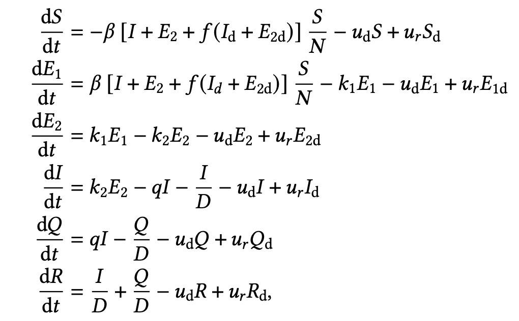
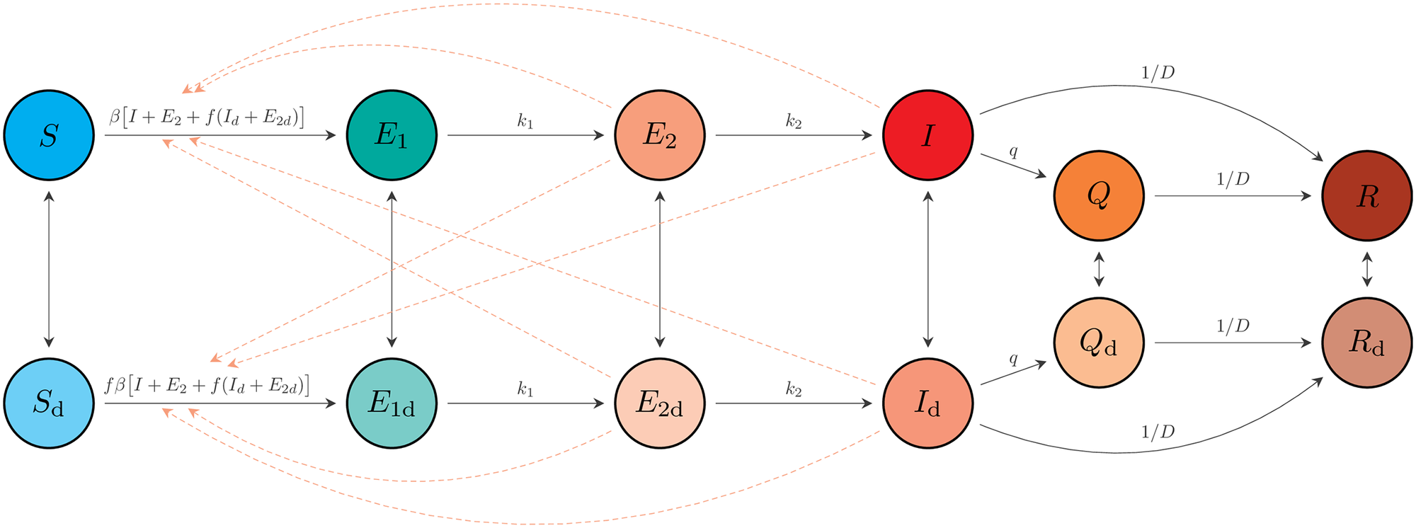
Rpackage: https://seananderson.github.io/covidseir/index.html- Paper link: https://doi.org/10.1371/journal.pcbi.1008274
Fit it to BC data and produce a forecast
samp_frac <- c(rep(0.14, 13), rep(0.21, 38), rep(0.37, nrow(early_bc) - 51))
f_seg <- with(early_bc, case_when(time_value == "2020-03-01" ~ 0, time_value >= "2020-06-01" ~ 3,
  time_value >= "2020-05-01" ~ 2, time_value > "2020-03-01" ~ 1))
fit <- covidseir::fit_seir(daily_cases = early_bc$cases,
                           f_seg = f_seg, # change points in transmission
                           samp_frac_fixed = samp_frac,  # fraction of infections that are tested
                           iter = 500, # number of posterior samples
                           fit_type = "optimizing") # for speed only
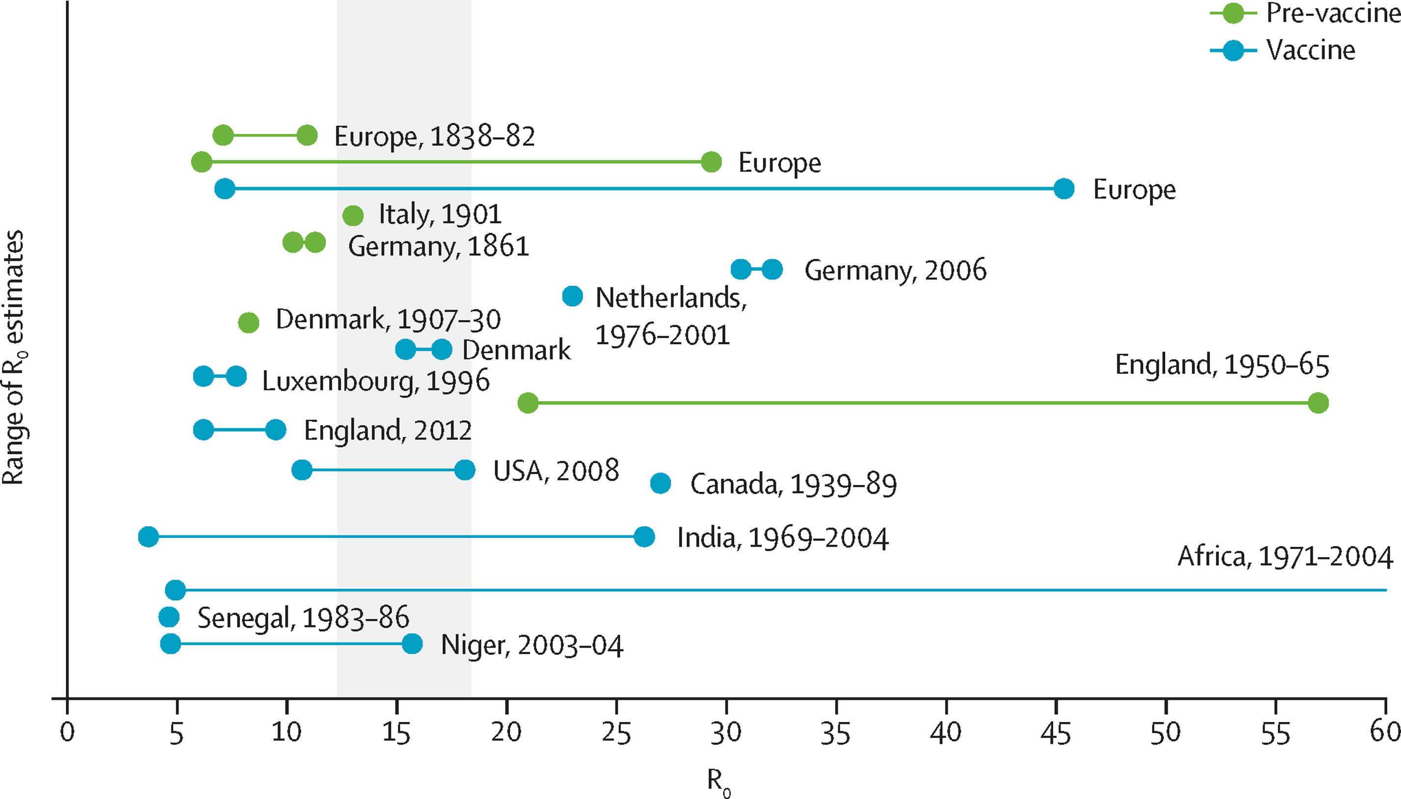
\(R_0\) basic reproduction number
Dates at least to Alfred Lotka (1920s) and others (Feller, Blackwell, etc.)
The expected number of secondary infections due to a primary infection
- \(R_0 < 1\) ⟹ the epidemic will die out
- \(R_0 > 1\) ⟹ the epidemic will grow until everyone is infected
\(R_0\) is entirely retrospective
It’s a property of the pathogen in a fully susceptible (infinite) population
Each outbreak is like a new sample
To estimate something like this from data, the “bonehead” way is to
- Wait until the epidemic is over (no more infections circulating)
- Contact trace the primary infection responsible for each secondary infection
- Take a sample average of the number caused by each primary
- Possibly repeat over many outbreaks
Of course no one actually does that
Lots of work on how to estimate \(R_0\)
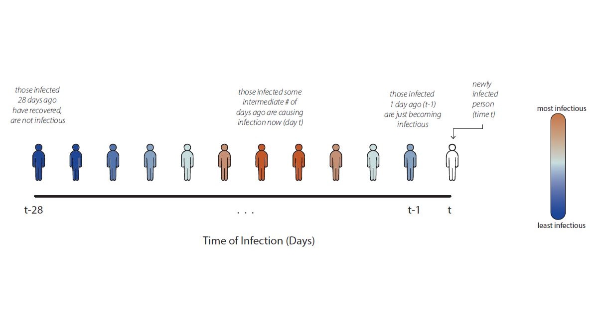
The generation interval distribution \(g(a)\)
\(R_t\) in compartmental models
There is an equivalence between a compartmental model and the renewal equation.
\[ \begin{aligned} R_0 &= \beta / \gamma\\ x_{t+1} &= \beta S_{t} \sum_{k = 0}^t \big[(1-\gamma)^{k}\big] x_{t-k} = R_0 S_{t} \sum_{k = 0}^t \big[\gamma(1-\gamma)^{k}\big] x_{t-k} = R_{t}\sum_{k = 0}^t g(k)x_{t-k} \end{aligned} \]

Data issues
\(x_t\) is Infections, but we don’t ever see those
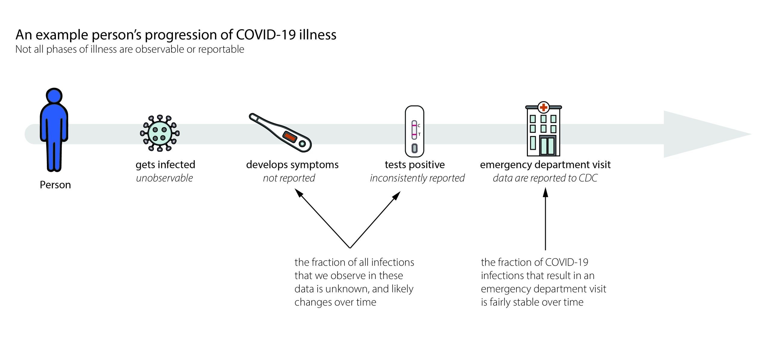
- Replace infections with cases
- Replace generation interval with serial interval
- Assume we have the serial interval
Serial interval distribution

Local adaptivity — \(\ell_1\) vs. \(\ell_2\)

Polynomial order, \(k=0\)
\[
\begin{aligned}
D^{(1)} &= \begin{bmatrix}
1 & -1 & & & & \\
& 1 & -1 & & & \\
& & & \ddots && \\
& & & & 1 & -1
\end{bmatrix} \\ \\
&\in \mathbb{R}^{(n-1)\times n}
\end{aligned}
\]

Polynomial order, \(k=1\)
\[
\begin{aligned}
D^{(2)} &= \begin{bmatrix}
1 & -2 & 1 & & & \\
& 1 & -2 & 1 & & \\
& & & \ddots && \\
& & & 1 & -2 & 1
\end{bmatrix} \\ \\
&= D^{(1)}D^{(1)}\\ \\
&\in \mathbb{R}^{(n-k-1)\times n}
\end{aligned}
\]

Polynomial order, \(k=2\)
\[
\begin{aligned}
D^{(3)} &= \begin{bmatrix}
-1 & 3 & -3 & 1 & & \\
& -1 & 3 & -3 &1 & \\
& & & \ddots && \\
& & -1 & 3 & -3 & 1
\end{bmatrix} \\ \\
&= D^{(1)}D^{(2)}\\ \\
&\in \mathbb{R}^{(n-k-1)\times n}
\end{aligned}
\]

Canadian Covid-19 cases

\(R_t\) for Canadian Covid-19 cases

Reconvolved Canadian Covid-19 cases

Example simulations for different methods

{rtestim} software
Guts are in C++ for speed
Lots of the usual S3 methods
Approximate “confidence” bands
\(\widehat{R}\) is a member of a function space
Arbitrary spacing of observations
Built-in cross validation
Time-varying delay distributions
{rtestim} software
Guts are in C++ for speed
Lots of the usual S3 methods
Approximate “confidence” bands
\(\widehat{R}\) is a member of a function space
Arbitrary spacing of observations
Built-in cross validation
Time-varying delay distributions

Approximation + Delta method gives
\[ \textrm{Var}(\widehat{R}) = \left(\textrm{diag}(\widehat{y}) + \lambda D^{\mathsf{T}}D\right)^{\dagger} \left(\frac{1}{\eta^2}\right) \]
{rtestim} software
Guts are in C++ for speed
Lots of the usual S3 methods
Approximate “confidence” bands
\(\widehat{R}\) is a member of a function space
Arbitrary spacing of observations
Built-in cross validation
Time-varying delay distributions

The solution is an element of the space of discrete splines of order \(k\) (Tibshirani, 2020)
- Lets us interpolate (and extrapolate) to off-observation points
- Lets us handle uneven spacing
{rtestim} software
Guts are in C++ for speed
Lots of the usual S3 methods
Approximate “confidence” bands
\(\widehat{R}\) is a member of a function space
Arbitrary spacing of observations
Built-in cross validation
Time-varying delay distributions


{rtestim} software

Wrapup and practice
- Basic compartmental modelling
- Difficulties in estimating compartmental models
- Standard epidemic parameters, \(R_0\)
- Discussion of \(R_t\) (model based vs nonparametric estimation)
- Some custom \(R_t\) software