CANSSI Prairies — Epi Forecasting Workshop 2025

Data Cleaning, Versioning, and Nowcasting

Lecture 2

Daniel J. McDonald

Outline

1. Warmup: Examining Snapshots
2. Signal processing with snapshots
3. Tracking Revisions
4. Nowcasting Using {epiprocess}
5. Nowcasting with Regression

Now that you have data, what do you do with it?

R4DS by Wickham, Çetinkaya-Rundel, and Grolemund

Complications

• Usually panel data (multiple locations at once)

• Usually accessing in real time

• Data have revisions

• Data are reported irregularly, NA’s are frequent

• Individual streams have high signal-to-noise ratio

Result: spend lots of time doing processing and dealing with corner behaviour

R packages we maintain to facilitate typical analyses

1 Warmup: Examining Snapshots

epi_df: snapshot of a data set

• a tibble with a couple of required columns, geo_value and time_value.
• arbitrary additional columns containing measured values, called signals
• additional keys that index subsets (health region, age_group, ethnicity, etc.)

epi_df

Represents a snapshot that contains the most up-to-date values of the signal variables, as of a given time.

epi_df: Snapshot of a dataset

can_edf <- can_cases_deaths |>
  rename(geo_value = region) |>
  as_epi_df(as_of = "2024-04-13", other_keys = "hr")
can_edf

An `epi_df` object, 150,951 x 5 with metadata:
* geo_type  = nation
* time_type = day
* other_keys = hr
* as_of     = 2024-04-13

# A tibble: 150,951 × 5
   geo_value hr       time_value cases deaths
 * <chr>     <chr>    <date>     <dbl>  <dbl>
 1 AB        South    2020-03-05     0      0
 2 AB        Calgary  2020-03-05     1      0
 3 AB        Central  2020-03-05     0      0
 4 AB        Edmonton 2020-03-05     0      0
 5 AB        North    2020-03-05     0      0
 6 AB        Other    2020-03-05     0      0
 7 AB        South    2020-03-06     0      0
 8 AB        Calgary  2020-03-06     0      0
 9 AB        Central  2020-03-06     0      0
10 AB        Edmonton 2020-03-06     0      0
# ℹ 150,941 more rows

Warm up: plotting

can_edf |>
  filter(geo_value == "MB") |>
  autoplot(cases, deaths) +
  scale_y_continuous(name = "", expand = expansion(c(0, .05))) + xlab("") + scale_color_delphi(name = "")

Weird reporting behaviour.

• MB stopped reporting deaths by HR.
• Put them all in “Other”
• Lots of missing values

Warm up: handling missingness

Two types of missing data

1. Explicit missingness means that there’s an NA
2. Implicit missingness means that a combination of time_value and geo_value is not in the data.

can_edf <- can_edf |>
  complete(time_value = full_seq(time_value, period = 1), fill = list(cases = 0, deaths = 0)) 
can_edf

An `epi_df` object, 150,951 x 5 with metadata:
* geo_type  = nation
* time_type = day
* other_keys = hr
* as_of     = 2024-04-13

# A tibble: 150,951 × 5
   time_value geo_value hr                               cases deaths
   <date>     <chr>     <chr>                            <dbl>  <dbl>
 1 2020-01-15 ON        Algoma                               0      0
 2 2020-01-15 ON        Brant                                0      0
 3 2020-01-15 ON        Durham                               0      0
 4 2020-01-15 ON        Grey Bruce                           0      0
 5 2020-01-15 ON        Haldimand-Norfolk                    0      0
 6 2020-01-15 ON        Haliburton, Kawartha, Pine Ridge     0      0
 7 2020-01-15 ON        Halton                               0      0
 8 2020-01-15 ON        Hamilton                             0      0
 9 2020-01-15 ON        Hastings and Prince Edward           0      0
10 2020-01-15 ON        Chatham-Kent                         0      0
# ℹ 150,941 more rows

Warm up: aggregating

can_prov <- can_edf |>
  sum_groups_epi_df(c(cases, deaths), group_cols = "geo_value")
can_prov

An `epi_df` object, 16,862 x 4 with metadata:
* geo_type  = nation
* time_type = day
* as_of     = 2024-04-13

# A tibble: 16,862 × 4
   geo_value time_value cases deaths
   <chr>     <date>     <dbl>  <dbl>
 1 AB        2020-03-05     1      0
 2 AB        2020-03-06     0      0
 3 AB        2020-03-07     1      0
 4 AB        2020-03-08     1      0
 5 AB        2020-03-09     4      0
 6 AB        2020-03-10     9      0
 7 AB        2020-03-11     7      0
 8 AB        2020-03-12     3      0
 9 AB        2020-03-13     8      0
10 AB        2020-03-14    22      0
# ℹ 16,852 more rows

Warm up: per capita scaling

can_prov <- can_prov |>
  inner_join(prov_pop, by = join_by(geo_value == region)) |>
  mutate(case_rate = cases / pop * 1e5, death_rate = deaths / pop * 1e6) |>
  select(-pop)

• Negative incidence is often due to cummulatives being differenced
• But sometimes due to correcting an error.
• With luck, the source would make an adjustment.

An `epi_df` object, 15 x 4 with metadata:
* geo_type  = nation
* time_type = day
* as_of     = 2024-04-13

# A tibble: 15 × 4
   geo_value time_value cases deaths
   <chr>     <date>     <dbl>  <dbl>
 1 AB        2020-10-08   186     -1
 2 AB        2021-04-26  1547     -7
 3 AB        2021-06-21    67     -2
 4 AB        2021-08-05   365     -4
 5 AB        2021-12-08   354     -1
 6 AB        2021-12-15   467     -1
 7 AB        2022-03-15   578    -12
 8 AB        2022-07-11   176     -4
 9 AB        2023-01-23    50     -5
10 AB        2023-03-13    60     -3
11 AB        2023-03-27    40   -700
12 NL        2021-08-25     2     -1
13 NS        2021-05-15    86     -1
14 SK        2020-12-28     0     -1
15 SK        2021-04-03   281     -1

2 Signal Processing with Snapshots

Examples of signal processing

1. Correlating signals across location or time
2. Computing growth rates
3. Detecting and removing outliers
4. Calculating summaries with rolling windows

Correlations at different lags (province-level)

cor0 <- epi_cor(can_prov, case_rate, death_rate, cor_by = geo_value)
cor21 <- epi_cor(can_prov, case_rate, death_rate, cor_by = geo_value, dt1 = -21)

• Are case and death rates linearly associated across all days for each geography?

• Deaths and cases likely not contemporaneous, expect cases to precede deaths.

Lag analysis more systematically

lags <- 0:35
can_lag_cors <- map(lags, \(l) epi_cor(can_prov, case_rate, death_rate, cor_by = geo_value, dt1 = -l)) |>
  set_names(lags) |> 
  list_rbind(names_to = "lag") |>
  summarize(mean_cor = mean(cor, na.rm = TRUE), .by = lag) |>
  mutate(lag = as.numeric(lag))

• Really strong weekly pattern.

• But we can fix that.

Quickly compute rolling functions by group

# trailing by default, new names are automatically created
can_prov <- epi_slide_mean(can_prov, c(case_rate, death_rate), .window_size = 7L)
can_lag_cors <- map(
  lags, 
  \(l) epi_cor(can_prov, case_rate_7dav, death_rate_7dav, cor_by = geo_value, dt1 = -l)
)

Notes on lagged correlations

Trailing average pushes the correlation backward

But weekly reporting aggregates incidence forward

These may roughly offset, but better if you know the probability of reports and deconvolve
more on this later

We were only averaging over 13 provinces + territories

Implicitly assuming that reporting / testing / disease behaviour is stable over 4 years

Compare to the US

# Only consider the 50 US states (no territories)
us_edf <- covid_case_death_rates |> filter(geo_value %in% tolower(state.abb)) 
cor0 <- epi_cor(us_edf, case_rate, death_rate, cor_by = geo_value)
cor21 <- epi_cor(us_edf, case_rate, death_rate, cor_by = geo_value, dt1 = -21)

Compare to the US

Aggregate cases tend to lead deaths by ≈23 days (arg max \(\rho\))

Same was true for Canada after smoothing, but lower correlation

Examining how correlations change over time

cor0 <- epi_cor(us_edf, case_rate, death_rate, cor_by = time_value, method = "kendall")
cor21 <- epi_cor(us_edf, case_rate, death_rate, cor_by = time_value, method = "kendall", dt1 = -21)

Compute growth rates

edfg <- filter(can_prov, geo_value %in% c("MB", "BC"), !is.na(case_rate_7dav)) |>
  mutate(gr_cases = growth_rate(case_rate_7dav, time_value, method = "linear_reg", h = 21L), .by = geo_value)

Outlier detection

outliers <- outliers |>
  mutate(detect_outlr_rm(time_value, cases), .by = geo_value)

Advanced sliding on an epi_df

• Compute rolling summaries of signals.
• These depend on the reference time
• Computed separately over geographies (and other groups).

epi_slide(
  .x,
  .f,
  ..., # for tidy-evaluation
  .window_size = NULL,
  .align = c("right", "center", "left"),
  .ref_time_values = NULL, # at which time values do I calculate the function
  .new_col_name = NULL, # add a new column with this name rather than the default
  .all_rows = FALSE # do return all available time_values, or only the ones with a result
)

.f “sees” a data set with a time value and other columns

That data is labeled with

1. A reference time (the time around which the window is taken)
2. A grouping key

• epi_slide() is very general, often too much so.
• We already saw the most common special case epi_slide_mean()
• For other common cases, there is epi_slide_opt()

Really ugly, but actually deployed slide functions

Function to flag outliers for corrections during late-2020 and early-2021

flag_covid_outliers <- function(signal, sig_cut = 2.75, size_cut = 20, sig_consec = 1.2) {
  signal <- rlang::enquo(signal)
  function(x, g, t) {
    .fns <- list(m = ~ mean(.x, na.rm = TRUE), med = ~ median(.x, na.rm = TRUE), 
                 sd = ~ sd(.x, na.rm = TRUE), mad = ~ median(abs(.x - median(.x)))
    )
    fs <- filter(x, time_value <= t) |> summarise(across(!!signal, .fns, .names = "{.fn}"))
    ss <- summarise(x, across(!!signal, .fns, .names = "{.fn}"))
    mutate(
      x, 
      ftstat = abs(!!signal - fs$med) / fs$sd, # mad in denominator is wrong scale, 
      ststat = abs(!!signal - ss$med) / ss$sd, # basically results in all the data flagged
      flag = 
        (abs(!!signal) > size_cut & !is.na(ststat) & ststat > sig_cut) | # best case
        (is.na(ststat) & abs(!!signal) > size_cut & !is.na(ftstat) & ftstat > sig_cut) | 
        # use filter if smoother is missing
        (!!signal < -size_cut & (!is.na(ststat) | !is.na(ftstat))), # big negative
      flag = flag | # these allow smaller values to also be outliers if they are consecutive
        (lead(flag) & !is.na(ststat) & ststat > sig_consec) | 
        (lag(flag) & !is.na(ststat) & ststat > sig_consec) |
        (lead(flag) & is.na(ststat) & ftstat > sig_consec) |
        (lag(flag) & is.na(ststat) & ftstat > sig_consec)
    ) |> filter(time_value == t) |> pull(flag)
  }
}

Really ugly, but actually deployed slide functions

Function to back distribute data randomly

corrections_multinom_roll <- function(x, excess, flag, time_value, max_lag = 30L, reweight = exp_w) {
  locs <- which(flag)
  if (length(locs) == 0) return(x)
  for (ii in locs) {
    if (ii <= max_lag) ii_lag <- seq_len(ii)
    else ii_lag <- seq(ii - max_lag + 1, ii)
    w <- reweight(length(ii_lag)) / length(ii_lag)
    x[ii] <- x[ii] - excess[ii]
    prop <- x[ii_lag] + sign(excess[ii]) * rmultinom(1, abs(excess[ii]), w)
    x[ii_lag] <- prop
  }
  x
}
exp_w <- function(n, std_decay = 30L, b0 = 8, a = exp(1) / 2){
  w <- (1:std_decay) / std_decay
  w <- tail(w, n)
  1 / (1 + exp(-w * b0 + a))
}

Roll our outlier detector, then calculate the corrections

corrections_df <- epi_slide(
  corrections_df, .align = "center", .window_size = 14L, .new_col_name = "flag",
  .f = flag_covid_outliers(deaths)
) |> mutate(corrected_deaths = corrections_multinom_roll(deaths, deaths, flag, time_value), .by = geo_value)

3 Tracking Revisions

epi_archive: Collection of epi_dfs

• Full version history of a data set
• Acts like a bunch of epi_df’s — but stored compactly
• Similar functionality as we saw but using only data that would have been available at the time

Revisions

Epidemiology data gets revised frequently.

• We may want to use the data as it looked in the past.
• or we may want to examine the history of revisions.

epi_archive: Collection of epi_dfs

Subset of daily COVID-19 doctor visits (Optum) and cases (JHU CSSE) from all U.S. states in archive format:

archive_cases_dv_subset_all_states

Summarize revision behaviour

revision_data <- revision_summary(archive_cases_dv_subset, case_rate_7d_av)
revision_data

Visualize revision patterns

Finalized data

• Counts are revised as time proceeds
• Want to know the final value
• Often not available until weeks/months later

Backcasting

At time \(t\), predict the final value for time \(t-h\), \(h < 0\)

Nowcasting

At time \(t\), predict the final value for time \(t\)

Forecasting

At time \(t\), predict the final value for time \(t+h\), \(h > 0\)

Sliding computations over archives

epix_slide(
  .x,
  .f,
  ...,
  .before = Inf,
  .versions = NULL,
  .new_col_name = NULL,
  .all_versions = FALSE
)

• To perform nowcasts we need to track how values get revised
• To evaluate forecasting models, we need to test them on the data we would have seen

4 Nowcasting Using {epiprocess}

Why this matters

• Every week BC CDC released COVID-19 hospitalization data.

• The following week, they revised the number upward (by ~25%) due to lagged reports.

Comparing preliminary to revised data often shows a decline.

Due to backfill

Backfill American edition - NCHS COVID-19 mortality

The revision triangle

• On day \(t\), predict the finalized value of signal \(y_t\)

• We may have a provisional value for \(y_t\) (subject to revision)

• Most likely, we only have provisional values for earlier dates

• We may only have “finalized” values for \(y_{t-s}\), \(s\gg0\)

Formal analysis of versioning behavior

Latency

the time difference between Reference Date and Initial Report Date

Backfill

the characteristics of updates after initial report (typical positive)

# same as before, but the NCHS data
revision_data <- revision_summary(nchs_archive, mortality, within_latest = .05, return_only_tibble = TRUE)
revision_data |> filter(geo_value == "ca", time_value %in% nchs_versions) |> print(width = 120)

# A tibble: 12 × 11
   time_value geo_value n_revisions min_lag max_lag  lag_near_latest spread
   <date>     <chr>           <dbl> <drtn>  <drtn>   <drtn>           <dbl>
 1 2024-01-07 ca                 19 1 weeks 47 weeks 10 weeks           170
 2 2024-01-14 ca                 11 1 weeks 21 weeks  6 weeks           144
 3 2024-01-21 ca                 12 1 weeks 29 weeks  5 weeks           111
 4 2024-01-28 ca                 13 1 weeks 23 weeks 10 weeks           113
 5 2024-02-04 ca                 13 1 weeks 42 weeks  9 weeks           102
 6 2024-02-11 ca                  9 1 weeks 14 weeks  5 weeks            89
 7 2024-02-18 ca                 10 1 weeks 37 weeks 11 weeks            81
 8 2024-02-25 ca                 10 1 weeks 53 weeks  8 weeks            74
 9 2024-03-03 ca                  8 1 weeks 14 weeks  8 weeks            46
10 2024-03-10 ca                 11 1 weeks 50 weeks  9 weeks            63
11 2024-03-17 ca                  7 1 weeks 25 weeks  8 weeks            50
12 2024-03-24 ca                  8 1 weeks 12 weeks 10 weeks            28
   rel_spread min_value max_value median_value
        <dbl>     <dbl>     <dbl>        <dbl>
 1      0.859        28       198        190. 
 2      0.754        47       191        184  
 3      0.730        41       152        148  
 4      0.785        31       144        136. 
 5      0.685        47       149        140. 
 6      0.856        15       104         99.5
 7      0.779        23       104         97  
 8      0.712        30       104         97  
 9      0.639        26        72         67  
10      0.851        11        74         70.5
11      0.769        15        65         60.5
12      0.683        13        41         37  

Revision pattern visualization

Building training data for nowcasting

• Can’t estimate any statistical model, unless I “see” the response
• The finalized value, is often very slow (~ 1 year for this signal)
• So a compromise is to use something close, here I’m using 95% of the finalized value

revision_ca <- filter(revision_data, geo_value == "ca")
revision_ca |> select(geo_value, time_value, lag_near_latest) |> slice_sample(n = 5)

# A tibble: 5 × 3
  geo_value time_value lag_near_latest
  <chr>     <date>     <drtn>         
1 ca        2021-07-11 16 weeks       
2 ca        2024-03-17  8 weeks       
3 ca        2021-04-04  9 weeks       
4 ca        2024-03-03  8 weeks       
5 ca        2023-03-19  6 weeks       

(lag_quantiles <- quantile(revision_data$lag_near_latest))

Time differences in weeks
  0%  25%  50%  75% 100% 
   1    6    8   13  156 

approx_final_lag <- lag_quantiles["75%"]

• Pretend that for time \(s\), the \(Y_s\) with version \(s +\) 13 weeks is “final”.
• At time \(t\), the most recent data in our training set will be 13 weeks old.

What about features?

Must use features that would have been available at test time.

Must have enough samples to ensure sensible estimation results.

1. provisional value(s) for time \(t\)
2. provisional value(s) for time \(t-\ell\)
3. exogenous signals that may be available

Potential model

Predictors are

• Provisional values for time \(t-\ell\), \(\ell =\) 1 week, 2 weeks when available
• Provisional \(Z_{t-k}\) for HHS/NHSN COVID-19 hospitalizations (these are daily, so different lags)

Exclude a potential predictor if it doesn’t have much training data available.

5 Nowcasting with Regression

Operationalizing

• Function needs to work on multiple nowcast dates
• Sometimes reporting changes, so we should adjust, not error
• If a predictor isn’t available, we remove it from the model and proceed
• Make sure we have “enough” training data to fit a model
• The nowcaster needs access to all versions prior to the nowcast date
• We want to retrain at every date: epix_slide(..., .all_versions = TRUE)
• Allow for linear regression or median regression

Big ugly function

• Goal: eventually refactor and put in {epipredict}

regression_nowcaster <- function(archive, model_settings, return_info = FALSE) {
  if (!inherits(archive, "epi_archive")) stop("`archive` isn't an `epi_archive`")
  if (n_distinct(archive$DT$geo_value) != 1L) stop("Expected exactly one unique `geo_value`")
  if (archive$time_type == "day") archive <- thin_daily_to_weekly_archive(archive)
  nowcast_date <- archive$versions_end
  target_time_value <- nowcast_date
  latest_edf <- archive |> epix_as_of(nowcast_date)

  predictor_descriptions <-
    latest_edf |>
    mutate(lag_days = as.integer(nowcast_date - time_value)) |>
    select(-c(geo_value, time_value)) |>
    pivot_longer(-lag_days, names_to = "varname", values_to = "value") |>
    drop_na(value) |>
    inner_join(model_settings$predictors, by = "varname", unmatched = "error") |>
    filter(abs(lag_days) <= max_abs_shift_days) |>
    arrange(varname, abs(lag_days)) |>
    group_by(varname) |>
    filter(seq_len(n()) <= max_n_shifts[[1]]) |>
    ungroup() |>
    mutate(predictor_name = paste0(varname, "_lag", lag_days, "_realtime")) |>
    select(varname, lag_days, predictor_name)

  predictor_edfs <- predictor_descriptions |>
    pmap(function(varname, lag_days, predictor_name) get_predictor_training_data(archive, varname, lag_days, predictor_name)) |>
    lapply(na.omit) |>
    keep(~ nrow(.x) >= model_settings$min_n_training_per_predictor)

  if (length(predictor_edfs) == 0) stop("Couldn't find acceptable predictors in the latest data.")

  predictors <- reduce(predictor_edfs, full_join, by = c("geo_value", "time_value"))
  target <- latest_edf |>
    filter(time_value <= max(time_value) - model_settings$days_until_target_semistable) |>
    select(geo_value, time_value, mortality_semistable = mortality)

  training_and_nowcast <- full_join(predictors, target, by = c("geo_value", "time_value"))

  training <- training_and_nowcast |>
    drop_na() |>
    slice_max(time_value, n = model_settings$max_n_training_intersection)

  nowcast_features <- training_and_nowcast |> filter(time_value == nowcast_date)

  form <- as.formula("mortality_semistable ~ .")
  fit_fun <- switch(
    model_settings$method,
    rq = function(x) { quantreg::rq(data = x, formula = form, tau = 0.5) },
    lm = function(x) { lm(formula = form, data = x) }
  )
  the_fit <- training |>
    select(any_of(predictor_descriptions$predictor_name), mortality_semistable) |>
    fit_fun()
      
  pred <- tibble(
    geo_value = "ca",
    nowcast_date = nowcast_date,
    target_date = target_time_value,
    prediction = unname(predict(the_fit, nowcast_features))
  )

  if (return_info) return(tibble(coefficients = list(coef(fit)), predictions = list(pred)))
  return(pred)
}

Model settings

We’ll compare 4 different configurations:

• Using lm() and only mortality predictors
• Using lm() with mortality and hospitalizations as a predictor
• Using rq() and only mortality predictors
• Using rq() with mortality and hospitalizations as a predictor

reg1_settings <- list(
  predictors = tribble(
    ~varname,    ~max_abs_shift_days, ~max_n_shifts,
    "mortality",                  35,             3,
    ),
  min_n_training_per_predictor = 30, # or else exclude predictor
  days_until_target_semistable = 7 * 7, # filter out unstable when training (and evaluating)
  min_n_training_intersection = 20, # or else raise error
  max_n_training_intersection = Inf # or else filter down rows
)

Comparison: linear regression

Comparison: quantile regression

Evaluations

Nowcaster	MAE	MAPE
Baseline	197.43	75.28
LinReg	172.03	106.74
LinReg + hosp	100.49	58.17
QuantReg	103.70	48.81
QuantReg + hosp	93.33	48.94

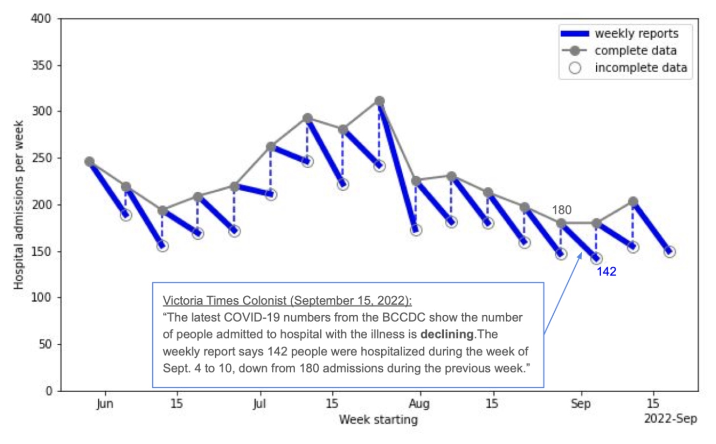
Aside on nowcasting

• To many Epis, nowcasting means estimate the instantaneous reproduction number, \(R_t\)

• Example: Reported COVID-19 cases in British Columbia (Jan. 2020 – Apr. 2023)

• More after lunch…

More practice with the worksheet

• Signal processing and exploratory data analysis

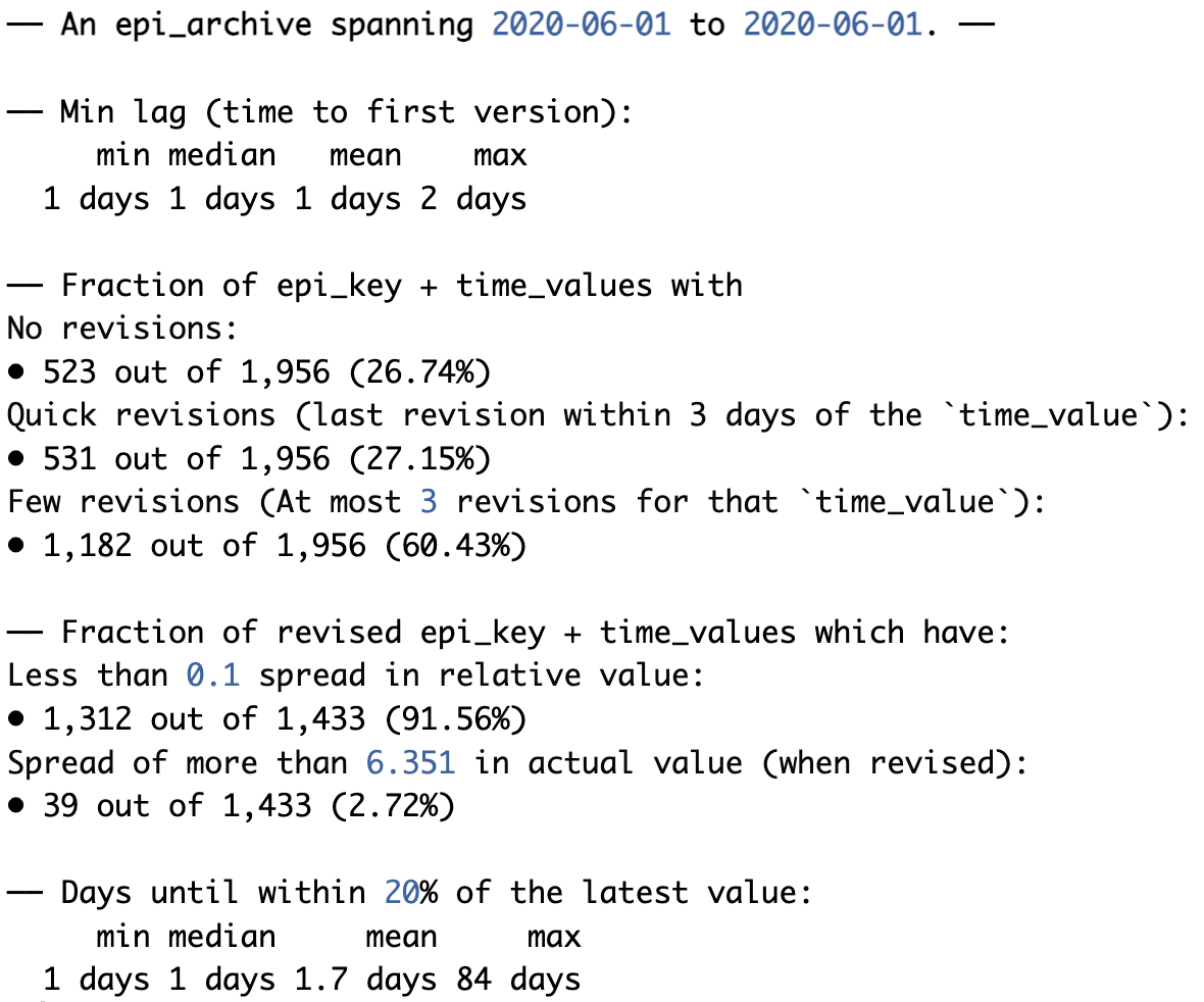
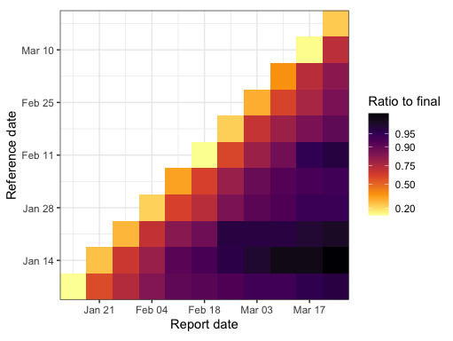
• Examining revision and latency patterns

• Thinking about the revision triangle and how to use it

• Basics of statistical nowcasting